1. 单变量时间序列预测基础

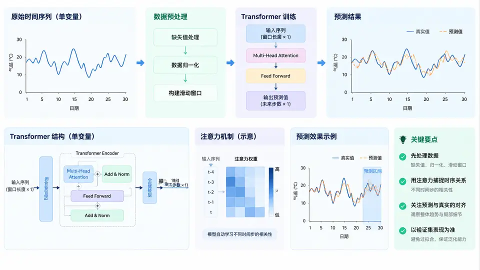
任务说明

本案例使用Transformer模型对单变量时间序列（每日最高气温）进行多步预测。输入过去48天的气温观测值，预测未来7天的气温走势。通过本案例掌握时间序列数据预处理（滑窗切分、归一化）、Transformer模型构建（位置编码、编码器-解码器结构）以及训练/验证的基本流程。

数据准备与预处理

采用北京2023年1月1日至12月31日的每日最高气温（单位：℃）作为实验数据。数据以CSV格式存储，包含date和temp两列。预处理流程如下：

读取CSV，提取气温序列；
使用MinMaxScaler将数据归一化至[0,1]区间；
以48个时间步为输入窗口、7个时间步为预测目标，构造监督学习样本；
按时间顺序划分训练集（前80%）和测试集（后20%），避免随机打乱造成数据泄漏。

Transformer模型定义

模型采用编码器-解码器架构：编码器接收48个时间步的输入序列，通过多头自注意力捕捉时间依赖；解码器以编码器输出为条件，通过全连接层直接生成7个未来值。关键超参数设置如下：

输入维度：1（单变量气温）；
模型维度 d_model=64，前馈网络维度 128；
注意力头数 4，编码器层数 2；
Dropout=0.1，用于缓解过拟合。

完整代码实现


import numpy as np
import pandas as pd
import torch
import torch.nn as nn
import math
from torch.utils.data import Dataset, DataLoader
from sklearn.preprocessing import MinMaxScaler

# ---------- 1. 数据加载与预处理 ----------
df = pd.read_csv('beijing_temp_2023.csv')
temps = df['temp'].values.astype(np.float32).reshape(-1, 1)

scaler = MinMaxScaler(feature_range=(0, 1))
temps_scaled = scaler.fit_transform(temps)

# 滑窗参数
SEQ_LEN = 48      # 输入窗口
PRED_LEN = 7      # 预测长度

def create_sequences(data, seq_len, pred_len):
    X, y = [], []
    for i in range(len(data) - seq_len - pred_len + 1):
        X.append(data[i:i+seq_len, 0])
        y.append(data[i+seq_len:i+seq_len+pred_len, 0])
    return np.array(X), np.array(y)

X, y = create_sequences(temps_scaled, SEQ_LEN, PRED_LEN)

# 按时间顺序划分（不打乱）
split_idx = int(len(X) * 0.8)
X_train, X_test = X[:split_idx], X[split_idx:]
y_train, y_test = y[:split_idx], y[split_idx:]

# 转换为PyTorch张量
X_train = torch.FloatTensor(X_train).unsqueeze(-1)  # (batch, seq, 1)
y_train = torch.FloatTensor(y_train)
X_test = torch.FloatTensor(X_test).unsqueeze(-1)
y_test = torch.FloatTensor(y_test)

# ---------- 2. 位置编码 ----------
class PositionalEncoding(nn.Module):
    def __init__(self, d_model, max_len=5000):
        super().__init__()
        pe = torch.zeros(max_len, d_model)
        position = torch.arange(0, max_len, dtype=torch.float).unsqueeze(1)
        div_term = torch.exp(torch.arange(0, d_model, 2).float() * (-math.log(10000.0) / d_model))
        pe[:, 0::2] = torch.sin(position * div_term)
        pe[:, 1::2] = torch.cos(position * div_term)
        self.register_buffer('pe', pe.unsqueeze(0))

    def forward(self, x):
        return x + self.pe[:, :x.size(1), :]

# ---------- 3. Transformer模型 ----------
class TransformerForecaster(nn.Module):
    def __init__(self, d_model=64, nhead=4, num_layers=2, dropout=0.1):
        super().__init__()
        self.input_proj = nn.Linear(1, d_model)
        self.pos_encoder = PositionalEncoding(d_model)
        encoder_layer = nn.TransformerEncoderLayer(
            d_model=d_model, nhead=nhead, dim_feedforward=128,
            dropout=dropout, batch_first=True
        )
        self.encoder = nn.TransformerEncoder(encoder_layer, num_layers=num_layers)
        self.decoder = nn.Sequential(
            nn.Linear(d_model, 32),
            nn.ReLU(),
            nn.Linear(32, PRED_LEN)
        )

    def forward(self, x):
        # x: (batch, seq_len, 1)
        x = self.input_proj(x)          # (batch, seq_len, d_model)
        x = self.pos_encoder(x)
        x = self.encoder(x)             # (batch, seq_len, d_model)
        x = x.mean(dim=1)               # 全局池化 -> (batch, d_model)
        out = self.decoder(x)           # (batch, PRED_LEN)
        return out

# ---------- 4. 训练配置 ----------
device = torch.device('cuda' if torch.cuda.is_available() else 'cpu')
model = TransformerForecaster().to(device)
criterion = nn.MSELoss()
optimizer = torch.optim.Adam(model.parameters(), lr=1e-3)

batch_size = 32
train_dataset = torch.utils.data.TensorDataset(X_train, y_train)
train_loader = DataLoader(train_dataset, batch_size=batch_size, shuffle=True)

# ---------- 5. 训练循环 ----------
epochs = 50
for epoch in range(epochs):
    model.train()
    total_loss = 0.0
    for batch_X, batch_y in train_loader:
        batch_X, batch_y = batch_X.to(device), batch_y.to(device)
        optimizer.zero_grad()
        pred = model(batch_X)
        loss = criterion(pred, batch_y)
        loss.backward()
        optimizer.step()
        total_loss += loss.item() * batch_X.size(0)
    avg_loss = total_loss / len(train_dataset)
    if (epoch + 1) % 10 == 0:
        print(f'Epoch [{epoch+1}/{epochs}], Loss: {avg_loss:.6f}')

# ---------- 6. 测试与反归一化 ----------
model.eval()
with torch.no_grad():
    test_pred = model(X_test.to(device)).cpu().numpy()
    test_true = y_test.numpy()

# 反归一化恢复真实温度
pred_temp = scaler.inverse_transform(test_pred.reshape(-1, 1)).reshape(-1, PRED_LEN)
true_temp = scaler.inverse_transform(test_true.reshape(-1, 1)).reshape(-1, PRED_LEN)

# 保存预测结果
np.save('test_predictions.npy', pred_temp)
np.save('test_ground_truth.npy', true_temp)
print('预测结果已保存至 test_predictions.npy')

运行与验证

运行方式：将上述代码保存为transformer_forecast.py，与数据文件beijing_temp_2023.csv置于同一目录，执行python transformer_forecast.py。依赖库包括numpy、pandas、torch、scikit-learn。

验证方法：训练过程中每10个epoch打印一次MSE损失，损失应呈下降趋势。训练结束后，程序输出测试集预测结果文件。可通过以下方式验证模型效果：

检查test_predictions.npy与test_ground_truth.npy形状均为(样本数, 7)；
计算测试集整体RMSE：rmse = np.sqrt(np.mean((pred_temp - true_temp)**2))，该值应明显小于直接使用历史均值预测的基准误差；
随机选取一个测试样本，绘制预测曲线与真实曲线对比，观察趋势是否吻合。

判定标准：训练损失收敛至0.01以下，且测试集RMSE低于3.5℃（以北京年温差约35℃为参照），即可认为模型已掌握基本的气温时序预测能力。

📚 课程目录