1. Introduction to data acquisition channel
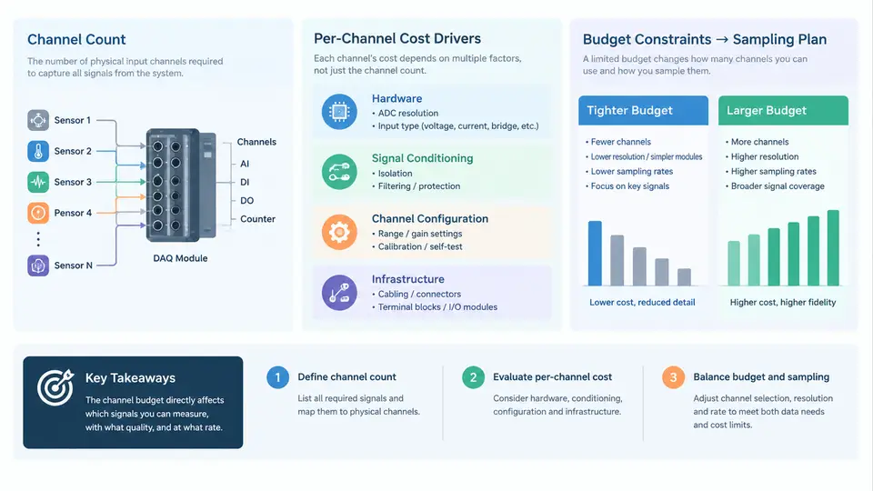
A data acquisition (DAQ) system rarely fails because the analog front end is fundamentally incapable. It fails because the channel budget was never made explicit. Engineers specify a sensor, choose a 24-bit ADC, and assume the measurement will be clean — only to discover at integration that the per-channel cost of isolation, filtering, and calibration has consumed the entire project allowance, forcing a reduction in channel count or a relaxation of the sampling plan. This chapter establishes the vocabulary and the arithmetic that prevent that outcome: what a channel budget is, which cost drivers dominate it, and how budget pressure propagates into the sampling plan.
What a Channel Budget Actually Contains
A channel budget is the allocation of a fixed resource — money, board area, power, firmware throughput, or engineering hours — across the channels of a DAQ system. In practice the binding constraint is usually monetary cost per channel at a given accuracy, but the same reasoning applies to any scarce resource. The budget has three layers that must be counted separately:
- Channel count (N): the number of independent measurement paths. Distinguish physical channels (sensor connections) from acquired channels (multiplexed inputs sharing one ADC) and simultaneous channels (each with dedicated conversion hardware). A 64-input system may be 64 physical, 16 acquired, and 4 simultaneous — three very different budgets.
- Per-channel cost drivers: the recurring cost of one complete signal path, from transducer terminals to digital samples.
- Fixed (shared) costs: chassis, backplane, controller, power supply, and software licences that do not scale with N but must be amortised across it.
The total budget is therefore not simply N × per-channel cost. A useful first-order model is:
Total cost  =  Fixed_cost  +  N × (Front_end + Conversion + Isolation + Calibration + Wiring)
Cost/channel =  Total cost / N
             =  Fixed_cost/N  +  per-channel recurring cost
The Fixed_cost/N term is why channel count and per-channel cost are coupled: doubling N dilutes the fixed cost but may also force a cheaper converter or a multiplexed topology, which changes the recurring term. Budgeting is an optimisation over both, not a multiplication.
The Per-Channel Cost Drivers
Walk one channel from the screw terminal to the digital output and the cost drivers appear in sequence. Each is a design decision with a price and an accuracy consequence.
| Driver | Typical cost impact | What it buys / costs in accuracy |
|---|---|---|
| Input protection & termination | Low | Survivability against miswiring; adds leakage and thermal EMF if poorly chosen |
| Amplification / PGA | Low–medium | Matches sensor span to ADC range; adds gain error and drift |
| Anti-alias filter | Medium | Order and cutoff set by sampling rate; higher order = more components per channel |
| Isolation | High | Breaks ground loops and protects personnel; dominates cost in industrial channels |
| ADC (shared vs dedicated) | Medium–high | Simultaneity and throughput; multiplexing trades cost for channel-to-channel skew |
| Calibration & traceability | Medium (recurring) | Removes offset/gain error; requires reference, fixtures, and periodic labour |
| Connectors, cabling, terminals | Low–medium | Often underestimated; scales linearly and is hard to reduce late |
Two observations matter for budgeting. First, the drivers are not independent: adding isolation usually forces a more expensive amplifier and a separate isolated supply, so the true incremental cost of isolation is a bundle, not a line item. Second, the largest driver is application-dependent. In a benchtop lab module, the ADC and reference dominate; in a 480 V motor test stand, isolation and protection dominate and can exceed the converter cost several times over.
How Budget Constraints Reshape the Sampling Plan
The sampling plan — which channels are sampled, how fast, with what simultaneity and filtering — is not chosen freely. It is the output of the budget. Three mechanisms connect them.
Throughput sharing. If N channels share one ADC of conversion rate fs_adc, the per-channel rate is at most fs_adc / N. A budget that funds one 1 MSPS converter for 32 channels yields 31.25 kSPS per channel — which may be below the Nyquist requirement for a vibration signal of interest. The budget has silently set the bandwidth.
Simultaneity versus cost. Dedicated per-channel converters remove skew but multiply converter and layout cost. Where phase relationships matter (power quality, multi-axis vibration), simultaneity is a requirement, not a luxury, and must be budgeted before channel count is fixed.
Filter order versus sample rate. A lower sampling rate demands a steeper anti-alias filter, which costs more per channel. Reducing the sample rate to save converter cost can therefore increase total cost. The trade must be evaluated jointly.
Worked Example: Budgeting a 16-Channel Strain Module
Consider a teaching example (all figures are illustrative assumptions, not measured results). A test rig needs 16 strain-gauge channels, 0–10 kHz bandwidth, simultaneous sampling, and 0.05 % accuracy. Assume:
Fixed cost (chassis, controller, PSU, software)   = $1,800
Per channel: bridge excitation + amp              = $22
             anti-alias filter (4th order)        = $14
             dedicated 24-bit ADC + reference     = $38
             terminals, wiring, connector         = $9
             calibration amortised over 3 years   = $6
Per-channel recurring                             = $89
Total = 1800 + 16 × 89 = $3,224   →   $201.50 / channel
Now suppose the project cap is $2,600. Options: (a) reduce to 12 channels — total $2,868, still over; (b) multiplex 16 channels onto 4 ADCs, saving roughly $38 × 12 ≈ $456 but introducing 3:1 skew and reducing per-channel rate to 250 kSPS — acceptable here since 10 kHz needs only ~25 kSPS; (c) drop isolation, which was not required in this benchtop case. Option (b) brings the total to about $2,768 before further trimming, and the sampling plan must now state the skew explicitly. The lesson: the budget decision is a sampling-plan decision, and it must be documented as one.
Documenting the Budget as a Design Artefact
Because the budget and the sampling plan are entangled, the budget should be a written artefact, not a spreadsheet held by one engineer. A minimal, directly usable record contains: the measurement requirement per channel (span, bandwidth, accuracy, simultaneity); the chosen topology (physical / acquired / simultaneous counts); the per-channel recurring cost broken down by driver; the fixed cost and the resulting cost per channel; and the explicit sampling-plan parameters that the budget permits — per-channel rate, filter order, and skew. When a later change arrives (a new sensor, a tighter accuracy target), its effect on the sampling plan is then visible immediately rather than discovered at integration.
With this foundation — channel count defined precisely, cost drivers enumerated, and the feedback from budget to sampling plan made explicit — the remaining chapters can treat each driver quantitatively. The next step in any real project is to convert the measurement requirement into a first-pass budget before a single component is selected.