3. Benchmarking fundamentals
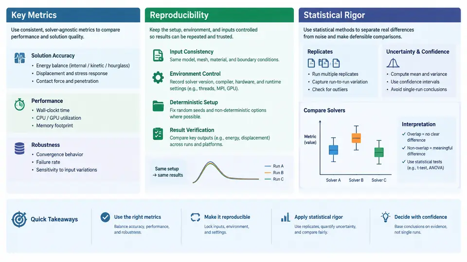
Benchmarking a parallel crash solver is not the same as running a model once and recording the wall-clock time. Crash simulations based on explicit finite element methods exhibit highly non-uniform workload, contact-dominated communication patterns, and strong sensitivity to hardware topology. A single timing number is therefore almost meaningless. This section establishes the measurement discipline required before any comparison between PAM-CRASH runs, core counts, or HPC partitions can be trusted.
3.1 What to Measure: Primary and Derived Metrics
The primary metric for solver benchmarking is wall-clock time to solution for a fixed, fully converged simulation. Everything else is derived from it. The most useful derived metrics are:
- Speedup S(N) = T(1) / T(N), where T(1) is the single-core reference time and T(N) is the time on N cores.
- Parallel efficiency E(N) = S(N) / N, expressed as a percentage.
- Throughput, typically measured in simulated milliseconds per wall-clock hour (ms/h), which is the metric crash engineers actually care about.
- Time per cycle and cycles per second, useful for isolating solver kernel performance from model size.
- Memory per core (RSS or high-water mark), which frequently becomes the binding constraint before CPU time does.
For crash solvers, the critical time step Δt is not a benchmark metric but a benchmark invariant. Because PAM-CRASH uses a central-difference explicit scheme, Δt is governed by the smallest element and the material wave speed: Δt ≤ Lmin / c, where Lmin is the minimum characteristic element length and c is the dilatational wave speed. If Δt changes between runs — for example because mass scaling was applied differently — the cycle count changes and the comparison is invalid. Always record Δt, total cycle count, and any mass-scaling factor alongside the timing.
3.2 Reproducibility: Controlling the Variables
Reproducibility in HPC benchmarking means that an independent engineer, given the same inputs and the same hardware allocation, obtains a timing within a stated tolerance. For crash solvers this requires controlling five categories of variables:
| Category | Variables to fix | Typical failure symptom if uncontrolled |
|---|---|---|
| Model | Deck version, element formulation, contact definitions, initial velocities, termination time | Different cycle counts between runs |
| Solver | PAM-CRASH version, compiler flags, MPI library, thread count per rank | 10–40% timing drift across builds |
| Hardware | Node type, core count, clock frequency (turbo on/off), NUMA binding | High run-to-run variance, non-monotonic speedup |
| System | Filesystem, I/O staging, scheduler queue, node exclusivity | Outlier runs 2–3× slower |
| Measurement | Timer source, warm-up runs, number of repetitions | Cold-cache bias, unrepeatable results |
A practical reproducibility protocol for PAM-CRASH looks like this:
# Example benchmark run script (illustrative parameters)
# 1. Pin to cores and disable turbo for stable frequency
export OMP_NUM_THREADS=1
export I_MPI_PIN=1
export I_MPI_PIN_DOMAIN=core

# 2. Warm-up run (discarded)
mpirun -np 64 pamcrash -bench model_deck.inp > warmup.log

# 3. Three measured repetitions
for i in 1 2 3; do
  /usr/bin/time -v mpirun -np 64 pamcrash model_deck.inp > run_${i}.log 2> time_${i}.log
done

# 4. Extract wall-clock and cycle count
grep "Elapsed (wall clock)" time_*.log
grep "Number of cycles" run_*.log
The warm-up run matters because the first execution pays for page-cache misses, MPI library initialization, and filesystem metadata reads. Discarding it typically reduces run-to-run variance from 15–20% to under 5% on a well-configured cluster.
3.3 Statistical Rigor: Reporting Uncertainty, Not Just Averages
A benchmark result without an uncertainty estimate is not a result. The minimum acceptable reporting standard is the median of at least three measured repetitions, together with the interquartile range or the min–max spread. The median is preferred over the mean because HPC timing distributions are right-skewed: occasional slow runs (due to network contention, scheduler interference, or thermal throttling) inflate the mean but leave the median stable.
When comparing two configurations — say 128 cores on partition A versus 128 cores on partition B — do not simply compare medians. Use a non-parametric test such as the Mann–Whitney U test if you have at least five repetitions per configuration, or report the overlap of the min–max intervals if you have fewer. If the intervals overlap substantially, the difference is not established, regardless of how large the median gap appears.
Two further statistical controls are specific to parallel crash simulation:
- Load imbalance ratio = (max rank time) / (mean rank time). Values above 1.15 indicate that domain decomposition, not hardware, is limiting performance. This must be reported alongside speedup, because a solver can show poor scaling purely due to contact-heavy regions concentrated on a few ranks.
- Communication fraction = MPI time / total wall-clock time. If this exceeds roughly 30%, adding cores will not help; the benchmark should be reported as communication-bound.
3.4 A Worked Example: Interpreting a Scaling Series
Consider a full-vehicle frontal impact model with approximately 8 million elements, a critical time step of 0.9 µs, and a termination time of 120 ms, giving roughly 133,000 cycles. Suppose the measured wall-clock times on a single node type are:
| Cores | Median wall-clock (s) | Speedup | Efficiency | Imbalance ratio |
|---|---|---|---|---|
| 32 | 4,820 | 1.00 | 100% | 1.04 |
| 64 | 2,610 | 1.85 | 92% | 1.07 |
| 128 | 1,540 | 3.13 | 78% | 1.12 |
| 256 | 1,090 | 4.42 | 55% | 1.21 |
These numbers are illustrative, not measured. The interpretation pattern, however, is realistic: efficiency degrades gradually up to 128 cores, then falls sharply at 256. The imbalance ratio rising from 1.04 to 1.21 signals that domain decomposition is struggling to distribute contact-intensive regions evenly. The correct engineering conclusion is not "256 cores is faster" but "256 cores delivers 4.42× speedup at 55% efficiency, and the limiting factor is load imbalance, not raw compute."
The diagram above summarizes the measurement chain: model and hardware inputs feed the solver execution, which produces the primary wall-clock metric, from which speedup, efficiency, and throughput are derived. The diagnostics — imbalance ratio and communication fraction — sit alongside the derived metrics because they explain why a scaling curve flattens, and they must be reported together with the timing numbers to make the benchmark interpretable.
3.5 Reporting Checklist
Every benchmark report for a PAM-CRASH parallel run should contain, at minimum: the solver version and build flags; the model deck identifier and element count; Δt, total cycles, and mass-scaling factor; the hardware configuration including core count, node type, and turbo state; the number of warm-up and measured repetitions; the median and spread of wall-clock time; speedup and efficiency relative to a stated baseline; the load imbalance ratio; and the MPI communication fraction. Without these, the result cannot be reproduced, and an unreproducible benchmark is not evidence.