1. PAM-CRASH solver architecture for HPC
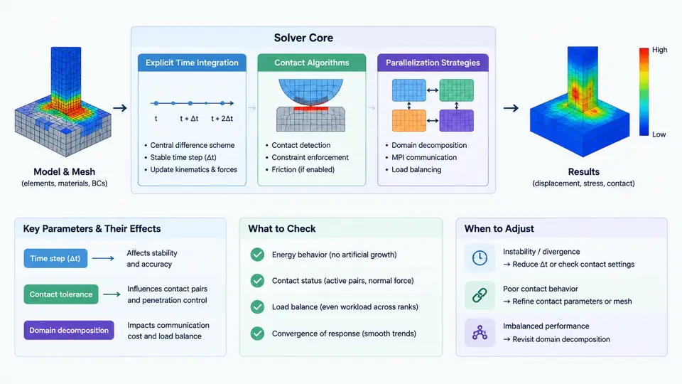
PAM-CRASH is a nonlinear explicit finite element solver widely used for crashworthiness, occupant safety, and impact simulation. Its architecture is shaped by a single dominant constraint: the explicit central-difference time integrator is conditionally stable, so the stable time step is bounded by the smallest element in the mesh. Everything else in the solver — contact search, element formulation, and parallel decomposition — is designed to keep that time step as large as possible while distributing the per-step work across many MPI ranks. Understanding this coupling is the prerequisite for interpreting any benchmark result later in this course.
Explicit time integration and the critical time step
The equation of motion solved at each step is M·a = F_ext − F_int, where the mass matrix M is lumped (diagonal). Because M is diagonal, no linear system is solved; accelerations are obtained by division, velocities and displacements are updated by central difference, and the whole step is embarrassingly parallel in principle. The stability limit for a linear element is:
Δt_crit = 2 / ω_max ≈ L_e / c
c = sqrt(E / ρ)          (bar wave speed)
where L_e is the characteristic element length and c the wave speed in the material. For a steel shell with E = 210 GPa, ρ = 7.8e-9 t/mm³, c ≈ 5.19e6 mm/s. A 5 mm shell element therefore gives Δt_crit ≈ 9.6e-7 s. A 100 ms crash event needs roughly 10⁵ steps. This is why a single distorted element of 0.5 mm can cut the global time step by a factor of ten and dominate wall-clock time — a failure mode you will meet repeatedly in benchmarking.
PAM-CRASH applies a safety factor (typically 0.9) and, optionally, mass scaling to raise Δt. Mass scaling adds non-physical inertia; it is acceptable only when the added mass stays below a few percent of the total and does not alter the energy balance. Always check the added-mass and energy-ratio output before trusting a scaled run.
Contact algorithms
Contact is the second architectural pillar and usually the largest consumer of CPU time. PAM-CRASH offers penalty-based and kinematic (constraint) methods. The penalty method computes a restoring force F = k·δ proportional to penetration δ, with stiffness derived from element properties:
k = f · (K · A²) / V (shell/solid penalty stiffness)
where K is the bulk modulus, A the contact area, V the element volume, and f a scale factor. Too small a penalty allows visible penetration; too large a penalty forces a smaller stable time step, because contact stiffness enters the stability estimate. This trade-off is the central tuning decision in crash models.
Search is organized in two phases. A broad phase uses a spatial bucket or bounding-box hierarchy to build a candidate pair list; a narrow phase performs exact node-to-segment or segment-to-segment tests. Self-contact and single-surface contact are the expensive cases because the candidate list cannot be precomputed once. Typical controls include CONTACT_THICKNESS, friction coefficients μ_static/μ_dynamic, and a search frequency that reuses the candidate list for several steps.
Parallelization strategy
PAM-CRASH parallelizes by domain decomposition: the mesh is partitioned into subdomains, one per MPI rank, using a graph partitioner that minimizes the edge cut (communication surface) while balancing element count. Each rank owns its elements and the nodes interior to it; nodes on subdomain boundaries are ghosted on neighbouring ranks. Per step, each rank computes internal forces locally, then exchanges ghost-node forces or velocities with neighbours, then advances its nodes.
Two costs scale differently. Computation scales as N_elements / P; communication scales with the interface area, roughly N_elements^(2/3) / P^(2/3) for a good partition. As P grows, communication and synchronization dominate, which is why speedup curves flatten. Contact adds a third term: contact pairs crossing subdomain boundaries require additional communication and, in the worst case, migration of contact segments.
Hybrid MPI+OpenMP is supported: MPI handles inter-node ghost exchange, OpenMP threads parallelize element loops within a rank. This reduces the number of ghost domains and often improves scaling on many-core nodes. The practical tuning knobs are the number of subdomains, the partitioning method, and the thread count per rank.
What this means for benchmarking
Three architectural facts drive every benchmark you will run. First, the time step is set by the worst element, so a benchmark that changes mesh quality changes the number of steps, not just the cost per step — always report both. Second, contact cost is not proportional to element count; it depends on how many surfaces are active and how the partition cuts them. Third, parallel efficiency is limited by the interface-to-volume ratio, so a fixed problem size will always show degrading speedup as P increases.
A minimal, reproducible scaling check on a 4-node cluster (32 cores per node) looks like this:
# Fixed problem, increasing core count
pamcrash -np 32  -i crash_model.inp -o run_p32
pamcrash -np 64  -i crash_model.inp -o run_p64
pamcrash -np 128 -i crash_model.inp -o run_p128
pamcrash -np 256 -i crash_model.inp -o run_p256

# Extract from the .out / timing file:
#   - number of time steps
#   - min / max / average Δt
#   - added mass (%)
#   - contact energy / internal energy
#   - wall-clock per 1000 steps
Expected observable behaviour: wall-clock per 1000 steps should fall roughly linearly up to 64–128 cores, then flatten. If it rises beyond that, check whether the partitioner produced a thin, high-interface decomposition, or whether contact search frequency is too high. If the number of steps changes between runs, the model is not being solved identically — investigate mass scaling or a changed Δt safety factor before comparing timings.
Key parameters to record for every benchmark
| Parameter | Typical value | Why it matters |
|---|---|---|
| Safety factor on Δt | 0.9 | Directly scales step count |
| Mass scaling target Δt | none / 1e-6 s | Changes physics if too aggressive |
| Penalty scale factor f | 0.1 – 1.0 | Trade-off: penetration vs. Δt |
| Contact search frequency | every 10–50 steps | Major cost driver |
| Subdomains (= MPI ranks) | 32 – 256 | Sets interface area |
| Threads per rank | 1 – 8 | Hybrid scaling behaviour |
With this architecture in mind — a conditionally stable explicit integrator, a penalty-based contact search whose stiffness feeds back into the time step, and a domain-decomposed parallel solver whose efficiency is bounded by interface communication — you are ready to design benchmarks that isolate each effect instead of confounding them.