3. Solver resource profiling

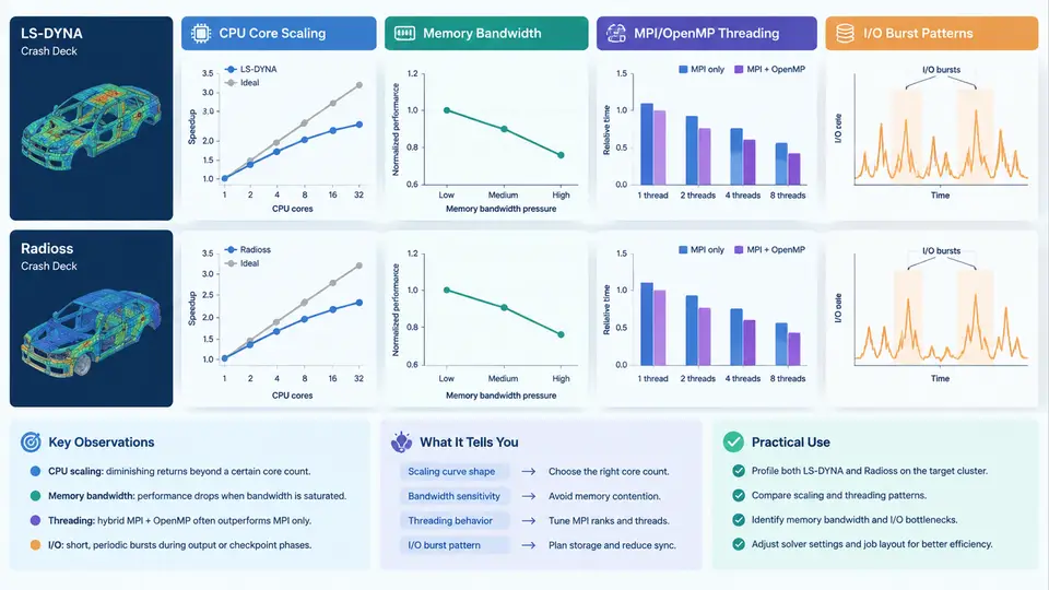
Before a crash solver is placed on a shared cluster, its resource signature must be measured rather than assumed. LS-DYNA and Radioss both expose knobs that change how work is partitioned, but the underlying hardware response is not linear. A deck that scales well to 32 cores may stall at 64, and a model that runs comfortably in 8 GB per rank may thrash once OpenMP threads share a single NUMA node. Profiling answers three questions: how many cores actually help, how much memory bandwidth each core consumes, and how the solver's threading and I/O behavior interacts with the scheduler's allocation.

Why profiling precedes scheduling

Shared clusters are heterogeneous. A node with 64 physical cores, two sockets, and 12 memory channels behaves differently from a 32-core single-socket node with 8 channels. If the scheduler treats them as interchangeable, jobs land on hardware that cannot feed them. Profiling produces a per-deck resource profile: a small set of numbers that the scheduler can use to select nodes, set rank counts, and predict wall-clock time. The profile is deck-specific because element count, contact density, material models, and output frequency all shift the balance between compute, memory, and I/O.

CPU core scaling

Core scaling is measured by running the same deck at increasing core counts and recording wall-clock time. The useful metric is speedup relative to a baseline, usually 8 or 16 cores, and parallel efficiency:

efficiency(N) = (T_base / T_N) / (N / N_base)

For a typical full-vehicle LS-DYNA deck, efficiency often holds above 0.85 up to 32 cores, then drops toward 0.6–0.7 at 64 cores as communication and memory contention grow. Radioss decks with heavy contact tend to degrade earlier because contact search is communication-intensive. The profiling run should use the production deck, not a reduced model, because scaling behavior depends on element distribution and contact topology.

A practical procedure: run the deck at 8, 16, 32, and 64 cores on a single node, record T_N from the solver's timing summary, and compute efficiency. If efficiency falls below 0.7, the additional cores are not worth the queue cost. The knee of the curve — the point where marginal speedup drops below roughly 0.5 per added core — defines the recommended maximum rank count for that deck.

Memory bandwidth sensitivity

Crash solvers are memory-bandwidth-bound more often than FLOP-bound. Each explicit time step reads element state, writes updated state, and performs contact queries. The arithmetic intensity is low, so performance tracks available bandwidth per core. On a dual-socket node, a rank pinned to one socket may see 60–70% of the bandwidth available to a rank spanning both, depending on the interconnect.

Measure bandwidth sensitivity by running the deck at a fixed core count while varying memory placement. Compare a run with all ranks on one socket against a run with ranks split evenly across sockets. If the split run is faster per rank, the deck is bandwidth-sensitive and should be scheduled on nodes with more channels per core. A simple proxy is to run STREAM or the solver's own memory benchmark on the target node and record GB/s per socket. Decks that show high bandwidth sensitivity should avoid oversubscribing cores per socket.

MPI and OpenMP threading behavior

LS-DYNA supports both pure MPI and hybrid MPI+OpenMP. Radioss similarly supports SMP and MPP variants. The choice affects scheduling because hybrid runs use fewer ranks but more threads per rank, which changes memory footprint and communication patterns.

Pure MPI: one rank per core, no shared-memory threading. Communication scales with rank count, and memory per rank is the full model divided by ranks. This is the default for most crash decks and is easiest to schedule.

Hybrid MPI+OpenMP: fewer ranks, each with multiple threads. Threads share the rank's memory, reducing total memory footprint, but OpenMP thread synchronization adds overhead. Hybrid is advantageous when the model is large and memory per rank is the binding constraint, or when the interconnect is slow relative to shared memory.

Profiling should record the rank-to-core mapping and thread affinity. On a dual-socket node, pinning one rank per physical core with OMP_NUM_THREADS=1 is the baseline. For hybrid, set OMP_NUM_THREADS to the number of cores per rank and use OMP_PROC_BIND=close to keep threads on the same socket. A common failure is threads migrating across sockets, which doubles memory latency and can cut performance by 30% or more.

I/O burst patterns

Crash decks produce bursty I/O. During initialization, the solver reads the input deck and writes restart files. During the run, d3plot or ANIM output is written at fixed intervals, and restart files are written periodically. These bursts can saturate the node's local disk or the shared filesystem, causing other jobs on the same node to stall.

Profile I/O by recording the size and frequency of output files. A typical LS-DYNA deck writing d3plot every 1 ms of simulated time may produce 2–5 GB per output step. If the run spans 100 ms, that is 200–500 GB of output. The scheduler must account for this: a job with heavy I/O should not share a node with another I/O-heavy job, and output should be directed to a filesystem with sufficient bandwidth.

Measure I/O burst duration by timing the write phases. If a write takes longer than the compute phase between writes, the job is I/O-bound and should be rescheduled or its output frequency reduced. For Radioss, the /ANIM and /RFILE output frequencies are the primary controls.

Building a reusable profile record

The output of profiling is a compact record that travels with the deck. A practical format is a single line per deck, stored alongside the input file or in the scheduler's job template:

deck: full_vehicle_v3.key
solver: LS-DYNA R13.1
baseline_cores: 16
max_efficient_cores: 32
efficiency_at_32: 0.87
efficiency_at_64: 0.62
memory_per_rank_gb: 6.4
bandwidth_sensitive: yes
recommended_mode: hybrid
omp_num_threads: 4
omp_proc_bind: close
io_burst_gb: 3.2
io_burst_interval_ms: 1.0
io_bound: no

This record lets the scheduler make three decisions without re-running the deck: how many cores to request, which node class to target, and whether to isolate the job from other I/O-heavy work. When the deck changes — mesh refinement, new contact definitions, different output frequency — the profile must be re-measured, because the knee and the I/O burst size both shift.

Common profiling pitfalls

• Using a reduced deck. Scaling behavior depends on element count and contact topology. A 100k-element model may scale to 64 cores; a 10M-element model may not.
• Ignoring thread affinity. Without OMP_PROC_BIND, OpenMP threads migrate across sockets, inflating memory latency and distorting the profile.
• Measuring only compute time. Wall-clock time includes I/O and initialization. A deck that looks compute-bound in the solver's CPU summary may be I/O-bound in wall-clock terms.
• Assuming node homogeneity. Two nodes with the same core count can differ in memory channels and interconnect. Profile on the node class the job will actually use.
• Profiling once. Solver versions, compiler flags, and MPI implementations change scaling. Re-profile after any of these change.

With a profile in hand, the scheduling problem becomes concrete: match the deck's core count, memory footprint, threading mode, and I/O burst to a node and a time window. The next chapter applies these profiles to the scheduler's placement and queueing logic.