1. Crash CAE workload landscape
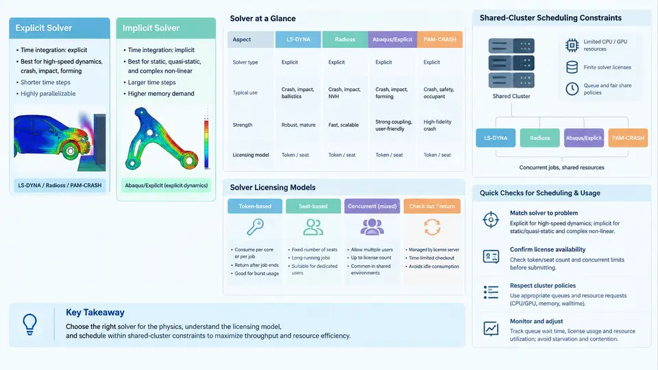
Crash CAE is not a single workload. It is a family of solver technologies with very different execution profiles, and those differences determine how they must be scheduled on a shared cluster. Before writing a single queue policy or license rule, you need a clear mental model of what each solver actually does at runtime: how long it runs, how many cores it can use, how it communicates, how it consumes licenses, and how it fails.
Explicit vs. Implicit: Two Different Machines
The first and most important split is between explicit and implicit time integration.
Explicit solvers (LS-DYNA, Radioss, Abaqus/Explicit, PAM-CRASH) advance the solution with a critical time step governed by the Courant condition. The step size is limited by the smallest element and the local wave speed, typically on the order of 0.1–1 µs for automotive crash models. A 150 ms frontal impact therefore requires roughly 150,000–1,500,000 time steps. There is no global matrix factorization, so each step is cheap and scales well across hundreds or thousands of cores. Memory per core is modest, but total memory scales with model size — a 20-million-element full-vehicle model can easily require 200–600 GB.
Implicit solvers (Abaqus/Standard, OptiStruct, Nastran) solve a global stiffness system at each increment. Steps are large, but each step involves sparse direct or iterative factorization, which is memory-intensive and scales less gracefully beyond a few hundred cores. Implicit jobs are common in crash-adjacent work: seat frame stiffness, closure durability, static equivalents, and preload states.
The practical scheduling consequence is direct: explicit jobs are throughput workloads that want many cores for a bounded wall-clock time; implicit jobs are capacity workloads that want large memory on fewer cores and can run for many hours.
Solver-by-Solver Execution Characteristics
LS-DYNA is the dominant explicit crash solver. Its MPP (Massively Parallel Processing) build uses domain decomposition with MPI; SMP (Shared Memory Parallel) uses OpenMP within a node. Most production crash runs use MPP across nodes. License consumption is per-core for MPP, which means a 512-core job consumes 512 license tokens — a hard constraint that often limits concurrency more than hardware does. LS-DYNA also supports *DATABASE_BINARY_D3PLOT output intervals that directly control I/O burst size.
Radioss (Altair) uses a hybrid MPI+OpenMP model (HMPP) and is known for strong scaling on structured and mixed meshes. Its licensing is also core-based, and it integrates tightly with PBS Professional, which is common in automotive HPC centers.
Abaqus/Explicit uses a domain-decomposition MPI model similar to LS-DYNA. Abaqus licensing uses a token pool where explicit and implicit jobs draw from the same pool at different rates, so a mixed workload can starve one solver type if tokens are not partitioned.
PAM-CRASH (ESI) is widely used in European OEM workflows, particularly for occupant and pedestrian protection. It supports both shared-memory and distributed-memory parallel execution and has its own license daemon, which must be accounted for separately in the scheduler.
Licensing Models and Their Scheduling Impact
License models are the single most underestimated constraint in crash CAE scheduling. Three patterns dominate:
- Per-core (per-seat) licensing: LS-DYNA MPP, Radioss HMPP. A job's license cost equals its core count. This creates a direct trade-off between job width and job concurrency.
- Token-pool licensing: Abaqus. Tokens are shared across solver types; a heavy implicit job can consume tokens that explicit jobs need.
- Named-user or node-locked: Some PAM-CRASH and specialty solver seats. These cannot be shared across the cluster and must be pinned to specific hosts.
The practical rule: never let the scheduler allocate more cores than you have license tokens for that solver. If you have 2,000 LS-DYNA MPP tokens and 5,000 physical cores, the effective ceiling is 2,000 cores of LS-DYNA work at any instant, regardless of idle hardware.
Shared-Cluster Scheduling Constraints in Practice
A shared cluster serves crash CAE alongside CFD, NVH, durability, and often non-CAE workloads. The scheduler must reconcile four competing pressures:
- Topology awareness: Explicit jobs scale best when ranks are placed within a low-latency fabric domain. Blind round-robin placement across islands can cut scaling efficiency by 20–40%.
- Memory fit: A 600 GB explicit job cannot be packed onto a node with 512 GB. The scheduler must enforce per-node memory limits and avoid oversubscription that triggers swapping.
- I/O staggering: Crash jobs write d3plot and restart files in bursts. If ten jobs write simultaneously to the same Lustre OST, aggregate throughput collapses. Staggering output intervals or using per-job scratch directories mitigates this.
- Fair-share and priority: A production crash run with a vehicle program deadline should preempt or outrank a parametric study. Fair-share weights by project, not by user, prevent one engineer from monopolizing the queue.
Assume a cluster with 4,000 cores, 2,000 LS-DYNA MPP tokens, 500 Abaqus tokens, and 200 TB Lustre scratch.
A typical frontal impact job: 256 cores, 350 GB, 8–14 h wall clock, 256 LS-DYNA tokens.
A typical implicit seat frame job: 64 cores, 180 GB, 6–20 h, 12 Abaqus tokens.
Maximum concurrent explicit jobs = min(4000/256, 2000/256) = min(15, 7) = 7 jobs.
Maximum concurrent implicit jobs = min(4000/64, 500/12) = min(62, 41) = 41 jobs.
But memory and I/O will bind first: 7 explicit jobs × 350 GB = 2.45 TB, which must fit across node memory; and 7 simultaneous d3plot writes can saturate Lustre. A realistic steady-state is 4–5 explicit jobs plus 15–20 implicit jobs, with output intervals staggered.
What to Check Before You Schedule Anything
When you inherit or design a crash CAE queue, verify these inputs first:
| Item | Why it matters | Typical value / check |
|---|---|---|
| Solver license count | Caps concurrency independent of hardware | lmstat -a -c 27000@license_host |
| Per-job core count | Determines packing and scaling | 128–512 for explicit, 32–128 for implicit |
| Peak memory per job | Prevents node oversubscription | From solver memory= setting or d3hsp |
| Scratch throughput | I/O bursts can stall all jobs | Measure with dd or ior |
| Interconnect topology | Affects MPI scaling | InfiniBand islands, NUMA domains |
| Project fair-share weights | Prevents queue monopolization | Set in scheduler config per project |
Error 302: license not available. This almost always means the scheduler allocated cores without checking token availability. Fix by adding a license-aware resource to the queue definition, not by reducing job size.
With this landscape established — explicit vs. implicit profiles, solver-specific execution behavior, license models, and the four scheduling pressures — the next chapters can move into concrete queue design, resource matching, and throughput tuning for production crash CAE.