3. Cluster sizing methodology
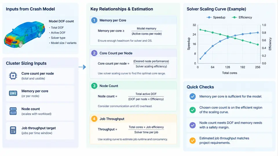
Sizing an HPC cluster for automotive crash CAE is not a matter of buying the largest machine the budget allows. It is a capacity-planning problem with three coupled unknowns: how many cores each job needs, how much memory each core must be paired with, and how many such jobs must run concurrently to meet the CAE team's delivery cadence. All three answers derive from two inputs that are measurable before any hardware is purchased: the model's degrees of freedom (DOF) and the solver's parallel scaling curve.
Step 1 — Establish the DOF budget per model
Crash models are dominated by shell elements, so DOF count is approximated as nodes × 6 (three translations plus three rotations per shell node), minus constrained DOF. A typical full-vehicle frontal impact model with 12 million nodes therefore carries roughly 72 million DOF. This number is the anchor for everything downstream: memory footprint, per-iteration cost, and the practical ceiling on useful core count.
Collect DOF counts for the entire model portfolio, not just the largest model. A realistic fleet for a vehicle program might look like this:
| Model class | Nodes | Approx. DOF | Typical run count per program |
|---|---|---|---|
| Subsystem / component | 0.5–2 M | 3–12 M | High (hundreds) |
| Full-vehicle frontal / side | 8–15 M | 48–90 M | Medium (tens) |
| Full-vehicle with occupant + barrier detail | 20–40 M | 120–240 M | Low (few) |
Note that DOF scales linearly with node count, but memory and runtime do not scale linearly with DOF — this is the crux of the sizing problem.
Step 2 — Derive memory per core from the implicit solver's working set
Crash solvers such as LS-DYNA, Radioss, or Abaqus/Explicit use an explicit time-integration scheme for the impact phase, but the initial stiffness matrix assembly, contact initialization, and any implicit or eigenvalue steps impose a substantial memory floor. The dominant memory consumers are:
- Element and node data: roughly 200–400 bytes per node for shell-heavy models, depending on the number of integration points and material history variables.
- Contact surfaces: penalty-based contact can add 50–150 bytes per contact node, and full-vehicle models often have 30–50% of nodes on contact surfaces.
- Solver working arrays: the explicit solver's internal vectors (velocity, acceleration, force) require approximately 100–200 bytes per DOF.
- MPP decomposition overhead: domain decomposition duplicates boundary nodes across ranks, adding 5–15% to the per-rank footprint.
A practical rule of thumb for explicit crash solvers is 1.5–2.5 GB of RAM per million DOF for the full model, distributed across all ranks. For a 72 M DOF full-vehicle model, the total memory footprint is therefore 110–180 GB. If the job is run on 192 cores, each core needs 0.6–0.9 GB — comfortably within a 2 GB/core node. But if the same job is run on 48 cores, each core needs 2.3–3.8 GB, which exceeds a 2 GB/core allocation and forces either a memory-optimized node or a higher core count.
Step 3 — Read the solver scaling curve to find the useful core ceiling
Parallel speedup in explicit crash solvers is sublinear because of three overheads: communication of boundary node data between domains, load imbalance from contact and element deletion, and serial sections such as contact initialization and output writing. A typical scaling curve for a 72 M DOF full-vehicle model on a modern InfiniBand-connected cluster might show:
| Cores | Wall-clock (hours) | Speedup vs. 48 cores | Parallel efficiency |
|---|---|---|---|
| 48 | 24.0 | 1.00× | 100% |
| 96 | 13.2 | 1.82× | 91% |
| 192 | 7.8 | 3.08× | 77% |
| 384 | 5.1 | 4.71× | 59% |
| 768 | 4.0 | 6.00× | 38% |
The knee of the curve — where efficiency drops below roughly 70–75% — is the practical core ceiling for that model. Here it lies between 192 and 384 cores. Beyond that point, adding cores consumes cluster capacity without proportional reduction in turnaround time, which directly harms throughput.
Step 4 — Estimate job throughput and node count
Throughput is the number of jobs completed per unit time, and it is what the CAE team actually delivers. The calculation is:
Required concurrent jobs = (jobs per program × programs per year) / (working hours per year × target utilization)

Example:
  Full-vehicle jobs per program:        40
  Programs per year:                     3
  Total full-vehicle jobs per year:     120
  Average wall-clock per job:           8 hours
  Working hours per year (24×7×0.85):  7,446 hours
  Required concurrent full-vehicle jobs: 120 × 8 / 7446 ≈ 0.13

  Subsystem jobs per program:           400
  Programs per year:                     3
  Total subsystem jobs per year:       1200
  Average wall-clock per job:           1.5 hours
  Required concurrent subsystem jobs:   1200 × 1.5 / 7446 ≈ 0.24
These numbers look small because they are averages. Real CAE demand is bursty: a program milestone can concentrate 30 full-vehicle runs into a two-week window. Sizing must account for peak concurrency, not annual average. A common approach is to size for the 90th-percentile demand week, which for this example might require 4–6 concurrent full-vehicle jobs and 15–20 concurrent subsystem jobs.
Translating concurrency into node count requires deciding the core allocation per job class. If full-vehicle jobs run at 192 cores and subsystem jobs at 48 cores, peak demand is:
Full-vehicle:  6 jobs × 192 cores = 1,152 cores
Subsystem:    20 jobs ×  48 cores =   960 cores
Total peak core demand:            2,112 cores
Add 15% headroom for scheduling gaps and failed jobs: 2,429 cores
With 128-core nodes, this rounds to 20 nodes — but only if memory per core is adequate. If the full-vehicle model needs 3 GB/core at 192 cores, the node must provide 384 GB for that job alone, and if two such jobs share a node, 768 GB. This is where the memory-per-core decision directly constrains node count and node configuration.
Step 5 — Validate the sizing against real queue behavior
After the cluster is in production, the sizing assumptions must be checked against actual scheduler data. The key metrics to monitor are:
- Job wait time by class: if full-vehicle jobs routinely wait more than 2–4 hours, peak concurrency was underestimated.
- Core utilization: sustained utilization below 60% suggests over-provisioning; above 90% with growing queues suggests under-provisioning.
- Memory high-water mark per job: if jobs are being killed by the OOM killer or swapping, the memory-per-core ratio is too thin for that model class.
- Scaling efficiency drift: as models grow, the efficiency knee shifts left. Re-measure scaling curves annually or when model size changes by more than 30%.
A practical validation loop is to run a representative full-vehicle model at 96, 192, and 384 cores, record wall-clock and peak memory, and compare against the sizing table. If the measured efficiency at 192 cores is below 70%, the useful core ceiling for that model is lower than assumed, and the node count must be increased to compensate — or the model must be decomposed differently.
The methodology is iterative: DOF counts drive memory and core estimates, scaling curves cap the useful core count, throughput requirements set the node count, and production monitoring closes the loop. Each input is measurable or estimable before purchase, which means the cluster can be sized with defensible numbers rather than vendor benchmarks or rules of thumb alone.