1. Crash CAE workload characterization
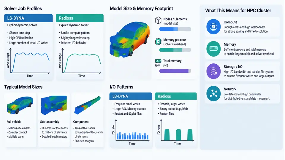
Before any cluster topology, scheduler policy, or storage tier is chosen, the crash CAE workload itself must be characterized. Automotive crash simulation is dominated by explicit finite element (FE) solvers — primarily LS-DYNA and Radioss — and their behavior differs fundamentally from implicit structural or CFD workloads. Explicit solvers advance the solution with a critical time step, perform no global matrix factorization, and instead spend nearly all compute time in element-level force calculations and contact detection. This single fact explains most of the cluster requirements that follow: high core counts per job, modest per-rank memory, low-latency interconnect, and bursty, write-heavy I/O.
Why Explicit Solvers Behave Differently
An explicit dynamic step solves M·a = F_ext − F_int with a lumped (diagonal) mass matrix, so the acceleration update is a vector operation with no linear solve. Stability is governed by the Courant condition, where the stable step is proportional to the smallest element characteristic length divided by the local sound speed. For a typical stamped steel body panel with a 5 mm shell element, the critical step is on the order of 0.5–1.0 µs. A 150 ms frontal impact therefore requires roughly 150,000–300,000 time steps. Because each step is cheap but there are hundreds of thousands of them, the workload is latency-sensitive and scales well across many ranks — provided contact and communication overhead stay controlled.
Two consequences matter for cluster design. First, jobs are usually run at high rank counts (64–1024 ranks) to shorten wall-clock time, so the cluster must deliver strong parallel efficiency at scale. Second, because there is no factorization, memory per rank is dominated by element, node, and contact data rather than a large sparse matrix — but total model memory still grows with model size, and contact surfaces can add substantial overhead.
Model Sizes and Memory Footprints
Automotive crash models range from component-level submodels to full-vehicle and full-body-in-white (BIW) models. The table below summarizes representative classes and their typical resource envelopes. These figures are illustrative planning values, not measured results from a specific site.
| Model class | Elements | Nodes | Typical ranks | Memory per rank | Wall-clock target |
|---|---|---|---|---|---|
| Component / subsystem | 0.5–2 M | 0.5–2 M | 16–64 | 1–2 GB | 0.5–2 h |
| Full vehicle (frontal) | 8–20 M | 8–20 M | 128–512 | 2–4 GB | 4–12 h |
| Full vehicle + occupant/restraint | 20–40 M | 20–40 M | 256–1024 | 3–6 GB | 8–24 h |
| Full BIW + closures, high fidelity | 40–80 M | 40–80 M | 512–2048 | 4–8 GB | 12–36 h |
A useful first-order memory estimate for LS-DYNA is roughly 1–2 GB per million solid/shell elements for the element and node data, plus contact and material state. Radioss follows a similar order. The practical planning rule is to size nodes so that a full-vehicle job fits with 30–40% headroom, because contact initialization and restart dumps create transient peaks.
I/O Patterns
Crash jobs are not continuously I/O-bound, but they produce sharp bursts. The dominant patterns are:
- Input deck read at startup: a single large keyword or Radioss input file (often 1–10 GB) read once, largely serialized, which stresses metadata and single-stream bandwidth.
- State and restart dumps: periodic
d3plot(LS-DYNA) or animation files (Radioss) written at intervals, each potentially tens of GB across a job, plusd3dump/restart files for recovery. - Contact and message passing: not file I/O, but the dominant inter-rank communication, which is why interconnect latency matters more than raw bandwidth for scaling.
- Post-processing reads: many analysts read the same result set concurrently, creating a read-heavy, random-access pattern best served by a parallel file system or a fast scratch tier.
From Workload to Cluster Requirements
The figure below maps the workload characteristics just described to the cluster resources they drive. Read it left to right: each workload property constrains a specific infrastructure decision.
Practical Characterization Workflow
To turn these generalities into site-specific numbers, run a short characterization pass before committing to a cluster design. A reproducible approach is:
- Select two or three representative decks: one component model, one full-vehicle frontal, and one high-fidelity BIW if available.
- Run each at three rank counts (e.g., 64, 256, 512) on the candidate hardware, recording wall-clock time, peak resident memory per rank, and MPI time fraction from the solver's timing summary.
- Compute parallel efficiency relative to the lowest rank count and identify the knee where efficiency drops below ~70%. That knee defines the practical maximum job size for the fabric and node architecture.
- Measure dump write throughput by timing a single
d3plotwrite and comparing it to the scratch tier's rated bandwidth.
For LS-DYNA, the timing summary at the end of d3hsp reports the breakdown between element processing, contact, and MPI. If MPI time exceeds roughly 20–25% of total, the interconnect or decomposition is the bottleneck, not CPU. For Radioss, the OUTPUT listing provides an analogous breakdown. Typical failure symptoms to watch for: jobs that scale well to 256 ranks but stall at 512 (fabric contention or load imbalance), and jobs that run fast but spend excessive time in dump writes (scratch tier undersized or shared with other traffic).
With the workload characterized — step counts, rank scaling, memory envelope, and I/O burst profile — the remaining cluster design decisions become traceable to measured requirements rather than vendor defaults. The next sections build on this characterization to specify compute nodes, interconnect, storage, and scheduling policy.