1. LS-DYNA multi-node scaling fundamentals

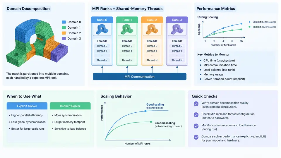
LS-DYNA is a hybrid-parallel finite element solver. When a model outgrows a single workstation, scaling to multiple nodes requires understanding how the solver partitions work across two orthogonal dimensions: MPI ranks that span nodes over a network, and shared-memory threads that run inside each rank on a single node. Getting good parallel efficiency means balancing both dimensions against the physics of the model, the memory bandwidth of the hardware, and the communication cost of the interconnect.

Domain Decomposition: How the Mesh Becomes Parallel Work

Before any MPI rank executes a time step, LS-DYNA decomposes the finite element mesh into contiguous subdomains, one per MPI rank. The decomposition is a graph-partitioning problem: minimize the number of elements whose nodes are shared across subdomains (the cut surface) while keeping each subdomain's element count roughly equal. LS-DYNA's default recursive coordinate bisection (RCB) and the optional METIS-based pfile decomposition both target this trade-off.

The cut surface matters because every node on a subdomain boundary must have its force and mass contributions exchanged with neighboring ranks each cycle. For explicit dynamics, this exchange is a latency-bound MPI halo swap; for implicit dynamics, it becomes a bandwidth-bound sparse matrix-vector product across ranks. A decomposition that produces 5% cut surface on a 10-million-element model is far better than one producing 20%, even if both have identical element counts per rank.

Two practical controls dominate decomposition quality:

• *CONTROL_MPP_DECOMPOSITION selects the partitioner and can bias toward minimizing communication (DECOMPOSITION=2 for METIS) or toward load balance.
• *CONTROL_MPP_DECOMPOSITION_TRANSFORMATION lets you weight specific parts or materials so that expensive regions (contact-heavy, thick-shell, or ALE) receive proportionally more elements per rank.

MPI Ranks vs. Shared-Memory Threads

LS-DYNA exposes two knobs that are often confused:

The product ncpu × OMP_NUM_THREADS should equal the number of physical cores you intend to use. Oversubscribing threads onto hyperthreads usually hurts explicit solver throughput because the memory subsystem is already saturated. A common starting point on a dual-socket node with 32 physical cores per socket is ncpu=2 and OMP_NUM_THREADS=32, giving one rank per socket and full socket-level threading.

Why not use 64 ranks of one thread each? Because MPI halo exchange cost grows with rank count, and on-node shared memory is far cheaper than inter-node messages. Why not use one rank with 64 threads? Because a single rank cannot use more than one node's memory, and thread scaling flattens once memory bandwidth is exhausted. The sweet spot is usually 1–4 ranks per node, each with 8–32 threads.

Performance Metrics That Actually Matter

Three numbers tell you whether scaling is working:

1. Speedup S(N) = T(1) / T(N) — wall-clock time on N cores divided into the single-core time. Report it against a fixed problem size (strong scaling) or fixed work per core (weak scaling).
2. Parallel efficiency E(N) = S(N) / N — the fraction of ideal speedup retained. Above 0.8 is good; below 0.5 means communication or load imbalance dominates.
3. Cycles per second (CPS) — LS-DYNA's own throughput metric, printed in the d3hsp file. It is the most direct indicator of explicit solver performance and is independent of problem size.

For implicit solvers, wall-clock per iteration and the number of iterations to convergence both matter. A parallel direct solver may show excellent speedup per iteration but require more iterations due to different reordering; always compare total time to solution, not per-iteration time.

# Example strong-scaling run on a 4-node cluster, 32 cores/node
mpirun -np 8 -x OMP_NUM_THREADS=16 ls-dyna_d R=model.k NCPU=8 OMP=16
# Observe in d3hsp:
#   "Number of MPI processes = 8"
#   "Number of threads per process = 16"
#   "Cycles per second = 1.24e+05"

Explicit vs. Implicit: Different Bottlenecks

Explicit LS-DYNA is dominated by element force computation and contact search, both of which are embarrassingly parallel within a subdomain. The parallel overhead is the halo exchange, which scales with cut-surface nodes and message latency. On InfiniBand or similar low-latency fabrics, explicit scaling to hundreds of ranks is routine. On 1 GbE, scaling stalls beyond 8–16 ranks because latency dominates.

Implicit LS-DYNA spends most time in the linear solver (sparse Cholesky or iterative). Here the bottleneck is memory bandwidth and the communication volume of the sparse matrix-vector product, not latency. Implicit scaling is more sensitive to the partitioner's ability to produce balanced subdomains with small separators, and it benefits more from threads than from additional ranks.

Putting It Together: A Scaling Diagnostic Workflow

When a model scales poorly, the diagnosis follows a predictable path. First, check the decomposition quality by inspecting the cut-surface node count printed in d3hsp under the decomposition summary. If the cut surface exceeds roughly 10% of total nodes, repartition with METIS or apply part weighting. Second, verify that ncpu × OMP_NUM_THREADS equals the physical core count and that ranks are pinned to NUMA domains using numactl or the scheduler's CPU binding. Third, run a short strong-scaling sweep (1, 2, 4, 8, 16 ranks) on a fixed model and plot efficiency; a sharp drop between two rank counts usually indicates the interconnect latency floor or a load-imbalance threshold.

For implicit models, add a fourth check: compare the number of solver iterations at each rank count. If iterations grow with ranks, the reordering is degrading preconditioner quality, and a different linear solver option (*CONTROL_IMPLICIT_SOLVER) may be needed.

The mental model to carry forward: domain decomposition defines what each rank owns, MPI ranks define how many network-separated workers exist, threads define how much on-node parallelism each worker exploits, and the three metrics — speedup, efficiency, and CPS — tell you whether the combination is working. Every subsequent scaling technique in this course builds on these four concepts.