3. Profiling crash simulation jobs
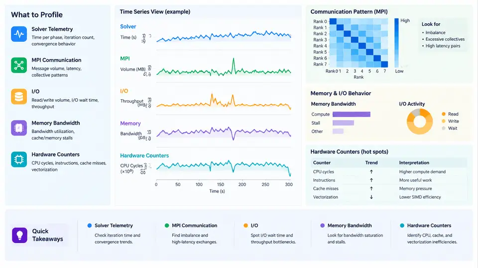
Crash simulation workloads built on LS-DYNA, Radioss, or PAM-CRASH are rarely limited by a single resource. A single explicit time step may be dominated by memory bandwidth, the next by MPI point-to-point latency, and the next by disk writes for d3plot or animation output. Effective optimization therefore begins with measurement, not with tuning. This chapter explains how to instrument a crash simulation job so that you can attribute wall-clock time to the solver kernel, MPI communication, I/O, memory traffic, and hardware-level stalls, and then decide which lever to pull.
What to Measure and Why
Four measurement layers are relevant to crash simulation:
- Solver telemetry — the internal timing and cycle reports emitted by the solver itself (LS-DYNA
d3hsp,messag, andglstat; Radioss*.outandTHfiles). These give element-cycle counts, contact time, and per-phase breakdowns. - MPI communication — message sizes, counts, and time spent in
MPI_Allreduce,MPI_Isend/Irecv, and neighbor exchange. Tools:mpiP,Score-P,Intel Trace Analyzer and Collector (ITAC),IPM. - I/O — read/write volume and latency for restart, d3plot, and binout. Tools:
Darshan,strace -c,iostat, Lustre/GPFS client counters. - Hardware counters — cache misses, memory bandwidth, vectorization efficiency, and stall reasons. Tools:
perf stat,likwid-perfctr,PAPI,Intel VTune,AMD uProf.
Each layer answers a different question. Solver telemetry tells you which phase is slow; MPI and I/O tools tell you where the time goes outside the compute kernel; hardware counters tell you why the kernel itself is slow.
Reading Solver Telemetry
In LS-DYNA, the messag file prints a per-cycle summary. A typical line looks like:
cycle   1  time 0.000E+00  dt 1.23E-07  elem  1.02E+06  mass 4.31E-02
cycle 500  time 6.15E-05  dt 1.18E-07  elem  1.02E+06  mass 4.31E-02
  contact  12.4%   element  61.2%   mpi  18.9%   io  4.1%   other  3.4%
The percentage breakdown is the fastest way to triage. If element dominates above ~70%, the kernel is compute- or memory-bound and hardware counters are the next step. If mpi exceeds ~25%, decomposition or communication pattern is the problem. If io spikes periodically, output frequency or file system contention is the cause.
MPI Communication Profiling
Crash simulations use domain decomposition, so each rank exchanges boundary node data with a small set of neighbors. The dominant patterns are:
- Neighbor exchange — point-to-point
MPI_Isend/Irecvbetween adjacent subdomains. Sensitive to message size and network latency. - Global reductions —
MPI_Allreducefor time-step, energy, and contact force sums. Sensitive to rank count and topology. - Collective I/O —
MPI_File_write_at_allfor d3plot. Sensitive to striping and file system.
To profile with mpiP, wrap the launch:
mpirun -np 256 mpiP --report=mpiP.txt \
  ls-dyna i=crash.k ncpu=256 memory=2000m
The resulting report lists each MPI call with total time, call count, and average message size. A healthy neighbor exchange shows average message sizes in the tens of kilobytes and time proportional to surface area. If MPI_Allreduce dominates, the reduction is likely on a critical path — check whether the solver supports hierarchical or topology-aware reductions.
I/O Profiling
Crash jobs write large binary state files. A 1M-element model may produce 5–20 GB of d3plot per output interval. Use Darshan by preloading it:
export LD_PRELOAD=/opt/darshan/lib/libdarshan.so
mpirun -np 256 ls-dyna i=crash.k ncpu=256
darshan-parser --file=crash.darshan > io_report.txt
Look for: total bytes written, number of small writes (a sign of poor buffering), and time spent in write vs open. If small writes dominate, increase the output buffer or switch to collective I/O. If open dominates, the file system metadata server is the bottleneck — reduce file count or use a single shared file.
Memory Bandwidth and Hardware Counters
Explicit crash solvers are memory-bandwidth-bound on modern CPUs. Each element update reads nodal coordinates, velocities, and stresses, then writes back forces. The arithmetic intensity is low (a few flops per byte), so DRAM bandwidth is often the ceiling.
Use perf stat to measure achieved bandwidth and cache behavior:
perf stat -e cycles,instructions,\
  cache-misses,cache-references,\
  LLC-load-misses,LLC-loads,\
  dram__bytes_read.all,dram__bytes_write.all \
  -p $(pgrep -n ls-dyna)
Key ratios to compute:
| Metric | Formula | Healthy range |
|---|---|---|
| IPC | instructions / cycles | 1.0–2.5 |
| LLC miss rate | LLC-load-misses / LLC-loads | < 20% |
| DRAM bandwidth | (bytes_read + bytes_write) / time | 60–85% of peak |
| Vectorization | vector instructions / total FP instructions | > 70% |
If DRAM bandwidth is above 80% of peak and IPC is below 1.0, the kernel is bandwidth-bound. Options: reduce memory footprint (single precision, element deletion), improve data layout (SoA instead of AoS), or use more ranks per node to increase memory-level parallelism.
perf stat per socket or use likwid-perfctr -C S0:0-63 to isolate. Aggregated numbers hide imbalance between sockets.Putting It Together: A Triage Workflow
The following SVG summarizes the decision path from a slow job to a specific optimization lever.
Practical Example: A 256-Rank LS-DYNA Job
Consider a 1.2M-element full-vehicle model running on 256 ranks across 8 nodes (32 ranks/node, dual-socket). The messag file reports:
contact 8.1% element 58.3% mpi 27.4% io 3.8% other 2.4%
MPI is above the 25% threshold. Running mpiP shows MPI_Allreduce consuming 62% of MPI time with an average of 4.1 ms per call, called 12,000 times. The reduction is for global time-step and energy. Two levers are available: (1) reduce reduction frequency by increasing the time-step interval between global syncs (if the solver exposes this), or (2) switch to a topology-aware reduction. After applying lever 1, MPI drops to 14% and total wall time improves by roughly 11%.
Next, hardware counters on the element phase show DRAM bandwidth at 78% of peak and LLC miss rate at 31%. The kernel is bandwidth-bound. Switching the model to single precision for the element loop (where the solver supports it) reduces memory traffic by ~40% and improves element time by ~18%. Combined, the two changes yield a ~26% wall-time reduction — but only because each was measured and attributed separately.
Checklist for a Profiling Run
- Run at least 500 cycles before reading telemetry.
- Capture
messag,glstat, andd3hspfor every run. - Enable mpiP or ITAC on at least one representative run per model.
- Preload Darshan for I/O-heavy runs (many output intervals).
- Run
perf statper socket for at least 60 seconds during steady state. - Record node count, ranks/node, MPI binding, and file system in a run log.
- Change one lever at a time; keep a before/after table.
With these measurements in hand, the next chapters on decomposition strategy, output tuning, and hardware selection become grounded in data rather than guesswork.