1. Crash simulation workloads on HPC
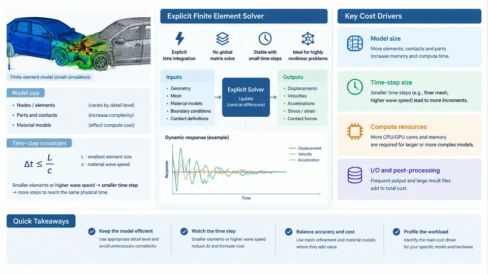
Crash simulation is one of the most demanding workloads in automotive CAE. Unlike static stiffness or modal analysis, a full-vehicle frontal impact must resolve large plastic deformation, contact between hundreds of parts, self-contact of folded sheet metal, and strain-rate-dependent material behavior — all within a physical event that lasts only 80–150 ms. The solver that dominates this domain is the explicit finite element (FE) solver, and understanding why it behaves the way it does is the foundation for every cost and energy optimization decision that follows in this course.
Why Explicit Integration Dominates Crash Analysis
An implicit solver solves the equilibrium equation K·u = f at every load step, requiring a global stiffness matrix factorization. For crash problems this is impractical: contact conditions change continuously, elements distort severely, and the stiffness matrix must be reassembled and refactorized many times per millisecond. The explicit solver instead advances the solution with the central-difference scheme:
u(n+1) = 2·u(n) − u(n−1) + Δt² · M⁻¹ · (F_ext − F_int)Because the mass matrix M is lumped (diagonal), no matrix inversion is needed — each element computes its own internal force and the update is a vector operation. This makes explicit solvers embarrassingly parallel and memory-light per element, but it introduces the single most important constraint in the entire workflow: the critical time step.
The Time-Step Constraint and the Courant Condition
The central-difference scheme is conditionally stable. The stable time step is governed by the Courant–Friedrichs–Lewy (CFL) condition, which for a solid element reduces to:
Δt_crit = L_e / c, c = sqrt(E / ρ)where L_e is the characteristic element length, c is the acoustic wave speed, E is Young's modulus, and ρ is density. For steel (E ≈ 210 GPa, ρ ≈ 7.85e-9 t/mm³), the wave speed is roughly 5.2 mm/ms. A 5 mm shell element therefore yields Δt_crit ≈ 0.96 µs. To simulate 100 ms of physical time, the solver must execute on the order of 100,000–200,000 time steps. This step count — not the model size alone — is what makes crash simulation expensive.
The practical consequence is that a single small element can dominate the entire run. If one element in a 10-million-element model has L_e = 0.5 mm, the global time step collapses to about 0.1 µs, and the step count increases tenfold. This is why mass scaling and element quality control are the first levers an engineer reaches for.
N_elements × N_steps. Reducing the minimum element size by 2× doubles the step count and therefore roughly doubles wall-clock time, even if the element count is unchanged.
Model Sizes in Realistic Crash Programs
Model size varies enormously by load case and fidelity target. The table below summarizes representative ranges observed in production automotive crash CAE. These are illustrative orders of magnitude, not measured results from a specific program.
| Load case | Typical element count | Typical min. element size | Physical duration | Approx. time steps |
|---|---|---|---|---|
| Full-vehicle frontal (50 km/h) | 8–20 M | 3–5 mm | 120 ms | ~150,000 |
| Side impact (pole / MDB) | 6–15 M | 3–5 mm | 100 ms | ~120,000 |
| Pedestrian head impact | 0.5–2 M | 1–2 mm | 30 ms | ~60,000 |
| Battery pack crush (EV) | 3–10 M | 2–4 mm | 80 ms | ~100,000 |
Two structural facts drive cost here. First, shell elements dominate — roughly 80–90% of the mesh — because body-in-white, closures, and battery enclosures are stamped or extruded thin-walled structures. Second, contact is everywhere: a full frontal model may define 300–800 contact interfaces, and contact search is a significant fraction of runtime, often 20–40%.
Where the Compute Time Actually Goes
Profiling a typical explicit crash run reveals a consistent breakdown. Element force calculation (strains, stresses, hourglass control) consumes the largest share, followed by contact detection and resolution, then equation-of-motion update and I/O. The relative weights shift with model characteristics: contact-heavy models with many small parts spend more time in contact; models with poor element quality spend more time in the smallest-element penalty.
Mass Scaling: The Primary Cost Lever
Because Δt_crit ∝ sqrt(ρ), artificially increasing the density of the smallest elements raises their critical time step. The standard technique is selective mass scaling: only elements below a target time step receive added mass, and the added mass is capped (typically 1–5% of total model mass) to avoid distorting inertia effects. A typical production setting targets a minimum time step of 0.8–1.0 µs, which often eliminates the handful of degenerate elements that would otherwise halve the global step.
The trade-off is physical fidelity. Adding mass to a 0.5 mm element in a crash-critical zone changes its inertia and can alter the deformation pattern. The correct workflow is to scale only in non-critical regions, verify that total added mass stays below the threshold, and confirm that the global time step is actually raised — not just the local one.
Practical Cost Estimation
A useful first-order estimate for planning purposes is:
Wall-clock ≈ (N_elements × N_steps × cost_per_element_step) / (N_cores × parallel_efficiency)For a 10 M element model at 150,000 steps on 512 cores, with a representative cost of ~1.5 µs per element-step per core and 70% parallel efficiency, the estimate is on the order of several hours. This is illustrative arithmetic, not a benchmark. The point is that the two dominant variables — element count and step count — are both controllable through mesh design and mass scaling, and both must be managed together.
What This Means for Optimization
Every subsequent chapter builds on this cost model. Reducing element count through submodeling or adaptive meshing attacks the first factor. Mass scaling, element quality improvement, and selective refinement attack the second. Contact simplification and output throttling reduce the per-step overhead. Energy optimization — the other half of this course — enters through CPU frequency scaling, memory bandwidth utilization, and the fact that explicit solvers are often memory-bandwidth-bound rather than compute-bound. Understanding the workload first is what makes those interventions measurable rather than speculative.