3. Infrastructure architecture for crash CA
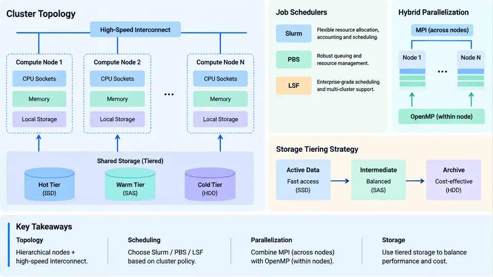
Crash CAE workloads—explicit LS-DYNA, Pam-Crash, or Radioss simulations—impose a distinctive combination of demands on HPC infrastructure: hundreds to thousands of cores per job, tightly coupled MPI communication at every time step, bursty I/O during d3plot and binout writes, and long-running jobs that must survive node failures without losing hours of computation. A well-architected crash CAE cluster is therefore not simply "a lot of CPUs." It is a carefully balanced system of interconnect topology, job scheduling policy, parallel decomposition strategy, and tiered storage. This section examines each layer and how they interact.
Cluster Topology and Interconnect
Crash simulation scales best when MPI ranks are placed on nodes with low-latency, high-bandwidth interconnect. Modern crash clusters typically use either InfiniBand HDR/NDR (200–400 Gb/s per port) or high-speed Ethernet (100–400 GbE with RoCEv2). The topology—fat-tree, dragonfly, or a 2-level rail-optimized fabric—determines bisection bandwidth and, critically, the cost of all-to-all and nearest-neighbor communication patterns that dominate explicit solvers.
A practical design principle: for a 500-node cluster running 64-core nodes, a non-blocking fat-tree with 1:1 oversubscription at the leaf and 2:1 at the spine is a common compromise. Rail-optimized topologies, where each node's NIC port i connects to leaf switch i, reduce hop count for the nearest-neighbor exchanges that dominate contact and element-force communication. The key metric to watch is MPI latency at 4 KB messages—crash solvers exchange small messages constantly, so sub-2 µs latency matters more than peak bandwidth for scaling beyond 512 cores.
Job Schedulers: Slurm, PBS, and LSF
The scheduler is the policy engine that decides which job runs where, for how long, and with what resources. All three major schedulers—Slurm, PBS Professional, and IBM Spectrum LSF—support the core features crash CAE needs: resource reservation, node exclusivity, job arrays, and preemption. The differences lie in configuration philosophy and ecosystem.
| Scheduler | Typical Crash CAE Use | Key Configuration |
|---|---|---|
| Slurm | Most common in new academic and automotive clusters | SelectType=select/cons_tres, TaskPlugin=task/affinity, topology-aware --switches |
| PBS Pro | Legacy automotive and aerospace environments | Node-locked licenses, place=scatter, queue-based priority |
| LSF | Large enterprise deployments with mixed workloads | Fair-share, bsub -n, resource reservation via brsvadd |
A representative Slurm submission for a 1024-core LS-DYNA job with hybrid MPI/OpenMP looks like this:
#!/bin/bash
#SBATCH --job-name=crash_full
#SBATCH --nodes=16
#SBATCH --ntasks-per-node=32
#SBATCH --cpus-per-task=2
#SBATCH --exclusive
#SBATCH --switches=1
#SBATCH --time=24:00:00
#SBATCH --output=crash_%j.log

export OMP_NUM_THREADS=$SLURM_CPUS_PER_TASK
export OMP_PROC_BIND=close
export OMP_PLACES=cores

srun --mpi=pmi2 --cpu-bind=cores \
  ls-dyna_smp_d_R11.1_linux_x86_64 \
  i=full_vehicle.k ncpu=$SLURM_CPUS_PER_TASK memory=2000m
The --switches=1 directive asks Slurm to place all 16 nodes under a single leaf switch, minimizing inter-node hop count. The --cpu-bind=cores and OMP_PROC_BIND=close settings pin each MPI rank to a physical core and its OpenMP threads to sibling cores, preventing thread migration that would destroy cache locality.
MPI/OpenMP Hybrid Parallelization
Crash solvers decompose the model spatially: each MPI rank owns a subset of elements, and at every time step ranks exchange nodal forces and velocities across partition boundaries. Pure MPI scaling degrades beyond ~512 ranks because the number of boundary nodes grows, and message-passing overhead dominates. Hybrid MPI/OpenMP reduces the number of MPI ranks while keeping the same core count, cutting communication volume and improving memory bandwidth utilization.
A practical rule for crash CAE: use 2–4 OpenMP threads per MPI rank on modern many-core nodes. For a 64-core node, 16 MPI ranks × 4 threads often outperforms 64 MPI ranks × 1 thread by 15–30% on contact-heavy models. The optimal ratio depends on model size per rank—if each rank owns fewer than ~50,000 elements, MPI overhead dominates and hybrid is essential.
ncpu set to the target rank count and inspect the d3hsp file for the "initialization" and "communication" timings. If communication exceeds 20% of total runtime, reduce MPI rank count and increase OpenMP threads.
Storage Tiering
Crash CAE generates two distinct I/O patterns: (1) large sequential writes of d3plot state files (often 10–100 GB per job) and (2) small random reads of input decks and restart files. A single storage tier cannot serve both efficiently. The standard architecture uses three tiers:
- Scratch (NVMe, node-local or parallel): Holds d3plot, binout, and restart files during the run. Node-local NVMe (3–8 TB per node) is fastest but not shared; a parallel filesystem like Lustre or BeeGFS with NVMe OSTs provides shared scratch at 100+ GB/s aggregate.
- Project (parallel HDD/SSD hybrid): Stores input decks, material libraries, and completed results. Lustre or GPFS with 10–20 GB/s aggregate bandwidth and POSIX semantics.
- Archive (object or tape-backed): Long-term retention of completed jobs, often via S3-compatible object storage or HSM. Not mounted directly by compute nodes.
The critical configuration detail is stripe alignment. For Lustre, set the stripe count to match the number of OSTs that can sustain the write bandwidth—typically 4–8 stripes for a 50 GB d3plot file. For node-local NVMe, ensure the solver writes to /scratch rather than the shared home directory, and stage results back to project storage after the run completes.
Putting It Together: A Reproducible Example
Consider a full-vehicle frontal impact model with 8 million elements, run on a 16-node cluster (64 cores per node, InfiniBand NDR). The target is a 120 ms simulation with a 1.2 µs time step—roughly 100,000 cycles.
Inputs: full_vehicle.k (2.1 GB), material library matlib.k, and a restart file from a previous 20 ms run. The model has 8M solid elements and 12M nodes.
Execution: Submit with 16 nodes × 32 MPI ranks × 2 OpenMP threads = 1024 cores. Set memory=2000m per rank (2 GB × 32 ranks = 64 GB per node, within the 256 GB node limit). Use --switches=1 to keep all nodes under one leaf switch.
Expected observable behavior: The d3hsp file reports initialization time (~45 s), then per-cycle communication time. On a well-tuned run, communication should be 8–12% of total runtime. If it exceeds 20%, the decomposition is too fine—reduce MPI ranks to 16 per node and increase OpenMP threads to 4.
Typical failure symptoms and troubleshooting:
- Job hangs at initialization: Check MPI fabric health with
ibstatand verify that all ranks can ping each other. A single bad HCA port can stall the entire job. - d3plot writes stall: If the solver pauses every few cycles, the scratch filesystem is saturated. Increase Lustre stripe count or move d3plot output to node-local NVMe.
- Poor scaling beyond 512 cores: Measure MPI latency with
osu_latency. If 4 KB latency exceeds 3 µs, the interconnect or rank placement is the bottleneck—enable rail-optimized routing or reduce rank count.
dt in the restart file matches the original run—a mismatch will cause immediate termination.
The architecture described here—rail-optimized interconnect, topology-aware scheduling, hybrid MPI/OpenMP decomposition, and three-tier storage—forms the foundation for reliable, scalable crash CAE. Each layer must be tuned in concert: a perfect scheduler cannot compensate for a saturated scratch filesystem, and the fastest storage cannot rescue a poorly decomposed MPI job. The next section builds on this foundation by examining how to monitor and diagnose these layers during production runs.