1. Crash CAE workload characterization
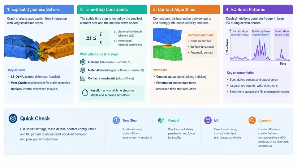
Crash simulation is not a generic HPC workload. Before designing fault tolerance for a crash CAE cluster, you must understand what the solver actually does per time step, why it cannot simply restart from an arbitrary point, and where the infrastructure is most likely to break. This chapter characterizes the workload produced by the three dominant explicit dynamics codes in automotive crash: LS-DYNA, Pam-Crash, and Radioss.
Explicit Dynamics: Why the Time Step Is the Whole Story
All three solvers integrate the equations of motion explicitly. There is no global stiffness matrix assembly and no linear system solve. Instead, each time step computes nodal accelerations from internal and external forces, then advances velocity and displacement:
a_n = M^-1 (F_ext - F_int)
v_(n+1/2) = v_(n-1/2) + a_n * dt
x_(n+1) = x_n + v_(n+1/2) * dt
Because the scheme is conditionally stable, the step size is bounded by the Courant–Friedrichs–Lewy condition. For a shell or solid element, the critical step is approximately the smallest element characteristic length divided by the dilatational wave speed:
dt_crit = L_e / c, c = sqrt(E / (rho * (1 - nu^2)))In practice, solvers apply a safety factor (LS-DYNA default TSSFAC = 0.9 for explicit solid/shell, 0.6 for some contact-dominated cases) and take the minimum over all elements. A typical automotive body-in-white model with 8–15 million elements and a 5 mm minimum shell edge length yields a stable step around 0.6–1.2 µs. A 120 ms frontal impact therefore requires roughly 100,000–200,000 cycles. This is the defining characteristic of the workload: a very large number of very small, tightly coupled steps.
The practical consequence for fault tolerance is severe. A single element with a collapsed or degenerate geometry can drive dt down by orders of magnitude, and the solver will report a mass-scaling or time-step warning. Monitoring dt and the controlling element ID is therefore a first-class health signal, not a diagnostic afterthought.
Contact Algorithms and Their Cost Profile
Contact is where crash simulation diverges most from other explicit workloads. LS-DYNA, Pam-Crash, and Radioss all support penalty-based and kinematic contact, but the dominant production choice for vehicle crash is penalty contact with a segment-based or node-to-surface formulation.
Penalty contact adds a stiffness term proportional to penetration depth. The contact stiffness k is derived from the slave and master segment bulk moduli and the segment area, scaled by a penalty factor SLSFAC (LS-DYNA default 0.1 for *CONTACT_AUTOMATIC_SURFACE_TO_SURFACE). If k is too large relative to the element stiffness, the contact stiffness itself can reduce the stable time step:
dt_contact = 2 * sqrt(m_slave / k_contact)This is why contact definitions directly affect runtime. A model with 200 contact interfaces, each with tens of thousands of segments, spends a substantial fraction of each cycle in contact search and force projection. Broad-phase search is typically bucket-sorted and only re-run when the search frequency (BSORT, default 25 cycles in LS-DYNA) elapses; narrow-phase and force computation run every cycle.
For infrastructure planning, the key numbers are: contact can consume 30–60% of per-cycle CPU time in a full-vehicle model, and contact state (active segments, penetration history, friction energy) is part of the restart state. A restart that loses contact history will produce non-physical force spikes in the first few cycles after resume.
I/O Burst Patterns
Crash solvers are not continuously I/O-bound, but they produce sharp, predictable bursts. Three output classes matter:
- State database (
d3plotin LS-DYNA,DSYin Pam-Crash,ANIMin Radioss): written everyDTinterval (commonly 0.5–2.0 ms of physical time). A 10 M-element model writes 200–800 MB per state, and a 120 ms job may produce 60–240 states. These writes are large, sequential, and bursty. - Restart files (
d3dump,RST): written at intervals or on demand. Size is comparable to a state file plus solver internal state. Restart write frequency is the single most important tunable for checkpoint cost. - Time-history and interface files (
binout,TH,glstat,matsum): small, written every cycle or every few cycles, and often on the master rank only.
The burst pattern is therefore: long compute-dominated phases punctuated by short, high-bandwidth write phases. On a shared parallel file system, synchronized state writes across hundreds of ranks can create metadata and bandwidth contention that stalls the solver. Staggering output across ranks or using a burst buffer is a common mitigation.
Code-Specific Differences That Affect Fault Tolerance
Although the three solvers share the explicit framework, their restart and checkpoint behavior differs in ways that matter for infrastructure design.
| Characteristic | LS-DYNA | Pam-Crash | Radioss |
|---|---|---|---|
| Restart file | d3dump | RST / RESTART | RST / ANIM |
| Restart granularity | Cycle or time interval | Time interval | Cycle or time interval |
| MPP decomposition | Domain decomposition, pfile | Domain decomposition | Domain decomposition, starter/engine |
| Contact restart fidelity | Full state in d3dump | Full state in RST | Full state in RST |
| Typical state size (10M elem) | 300–800 MB | 250–700 MB | 300–750 MB |
| Output frequency control | *DATABASE_BINARY_D3PLOT | DT in /RUN | /TFILE / /ANIM |
The practical implication is that a fault-tolerant layer must be solver-aware. A generic checkpoint/restart at the OS or MPI level will capture memory and file state, but it will not know whether the contact history in the restart file is consistent with the current cycle. For LS-DYNA MPP, the d3dump file is the authoritative restart artifact; for Radioss, the RST plus the starter input define the restart point. Any fault-tolerance design must align its checkpoint cadence with the solver's own restart cadence, not impose an arbitrary interval.
What This Means for Infrastructure Design
Three workload properties drive every subsequent design decision in this course:
- Long-running, tightly coupled cycles. A 24–72 hour job with 100k+ cycles means that losing 30 minutes of work is acceptable, but losing contact state is not. Checkpoint frequency must be tuned to the cost of recomputation versus the cost of writing.
- Bursty, synchronized I/O. State writes from hundreds of ranks at the same physical time create contention. Fault-tolerant storage must absorb these bursts without stalling the solver.
- Solver-specific restart semantics. The fault-tolerance layer cannot treat the solver as a black box. It must understand which files constitute a valid restart point and when they are consistent.
dt and its controlling element, the per-cycle wall time split between contact and non-contact, and the size and frequency of state database writes. These three numbers determine checkpoint cost, storage bandwidth requirements, and the maximum tolerable checkpoint interval.
With this characterization in hand, the next chapters can address how to build checkpointing, replication, and recovery mechanisms that respect the solver's actual behavior rather than fighting it.