3. Mapping and interpolation
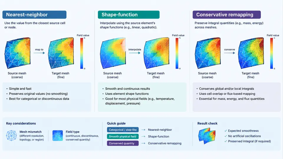
Once two solvers have produced results on their own meshes, the comparison problem reduces to a single question: how do we transfer a field defined on mesh A onto mesh B without inventing physics? This is the mapping (or remapping) step, and it is the most error-prone part of any CAE harmonization workflow. A structural solver may deliver nodal displacements on a coarse quadratic tetrahedral mesh, while a CFD solver reports surface pressure on a fine triangular surface mesh. Neither mesh knows about the other. The mapping operator is the only bridge between them, and its choice determines whether your comparison is meaningful or merely colorful.
Why the transfer operator matters
Every remapping scheme is an approximation. The goal is not to eliminate error but to control it in a way that is consistent with the physics you are comparing. Three families dominate engineering practice:
- Nearest-neighbor — assign each target point the value of the closest source point.
- Shape-function (nodal) interpolation — evaluate the source element's basis functions at the target point's parametric coordinates.
- Conservative remapping — integrate the source field over the intersection of source and target control volumes so that the total (mass, flux, energy) is preserved.
The wrong choice produces characteristic artifacts: a pressure field that looks blocky, a heat flux that gains or loses energy at the interface, or a stress field that oscillates near mesh transitions. Recognizing these signatures is how you diagnose a bad mapping.
Nearest-neighbor: fast, robust, and blunt
Nearest-neighbor (NN) mapping finds, for each target node xt, the source node xs minimizing ‖xt − xs‖ and copies its value. It requires no element connectivity on the source side, which makes it the fallback when meshes are non-conforming, partially overlapping, or topologically incompatible.
The cost is accuracy. NN is only first-order and piecewise-constant: the mapped field inherits the source mesh's nodal spacing as a visible "staircase." For a 2 mm source mesh mapped onto a 0.5 mm target mesh, the target field will show 2 mm plateaus. NN is acceptable for categorical data (material IDs, region flags) or for a quick sanity check, but it should never be used to compare gradients or peak values.
Shape-function interpolation: accurate inside elements
Shape-function interpolation is the natural choice when the source mesh is a proper finite-element mesh. For each target point, you locate the containing source element, compute the local (parametric) coordinates ξ, η, ζ, evaluate the element shape functions Ni(ξ, η, ζ), and form the interpolated value:
u_target = Σ_i N_i(ξ, η, ζ) · u_source_iFor a linear tetrahedron, the shape functions are the barycentric coordinates; for a hexahedron, the standard trilinear functions. The result is second-order accurate inside the element and reproduces linear fields exactly — a property called linear precision. This is why shape-function mapping is the default for displacement, temperature, and other smooth nodal fields.
The practical difficulty is point location. Finding which source element contains a given target point is the dominant cost, and it fails at boundaries. A target point that falls outside the source domain — common when meshes have different extents — has no valid element. Robust implementations use a bounding-volume hierarchy for the search and a fallback (usually NN) for exterior points, with a warning that the extrapolation is not physically valid.
Conservative remapping: preserving the integral
When the quantity being transferred is a conserved physical quantity — mass flux, heat flow, momentum — the mapping must satisfy a discrete conservation law. Conservative remapping enforces:
Σ_target V_t · u_t = Σ_source V_s · u_swhere V denotes control-volume (or area) weights. The standard approach is supermesh construction: overlay the source and target meshes, compute the polygon/polyhedron of intersection for every overlapping pair, and distribute the source contribution proportionally to the intersection measure. Each target cell then receives a weighted sum of the source cells it overlaps.
Conservative remapping is more expensive — supermesh generation is the bottleneck — and it is only first-order accurate for cell-centered data unless you add gradient reconstruction. But it is the only scheme that guarantees the global balance your solver's physics depends on. For conjugate heat transfer, fluid–structure interaction, and any coupled analysis, this is non-negotiable.
Choosing the right scheme
| Scheme | Accuracy | Conservation | Best for | Typical failure |
|---|---|---|---|---|
| Nearest-neighbor | 1st order, piecewise constant | No | Categorical data, fallback | Staircase artifacts, integral drift |
| Shape-function | 2nd order, linear precision | No | Smooth nodal fields (displacement, T) | Extrapolation error outside source domain |
| Conservative | 1st order (cell-centered) | Yes | Flux, mass, energy, coupled physics | Supermesh cost, non-convex intersections |
A practical decision rule: if the quantity has a physical conservation law, use conservative remapping. If it is a smooth nodal field and the meshes overlap well, use shape-function interpolation. Use nearest-neighbor only when nothing else is available or the data is categorical.
Worked example: mapping surface pressure
Consider a CFD surface pressure field on a fine triangular mesh (mean edge length 0.8 mm) being mapped onto a coarser structural surface mesh (mean edge length 3 mm) for a one-way FSI load transfer. The pressure is a flux-like quantity acting on the structural surface, so the correct choice is conservative remapping.
- Inputs: source mesh with 142,000 triangular faces and nodal pressure values; target mesh with 9,800 quadrilateral faces; both surfaces nominally coincident but with a 0.05 mm offset from CAD tolerance.
- Preprocessing: project target face centroids onto the source surface along the average normal to close the 0.05 mm gap. Record the projection distance; values above 0.1 mm indicate a geometry mismatch that must be fixed before mapping.
- Supermesh: for each target face, find overlapping source faces via a bounding-volume hierarchy, compute intersection polygons, and accumulate the area-weighted pressure.
- Output: target face pressure values plus a per-face coverage fraction. Faces with coverage below 0.95 are flagged.
- Verification: compare Σ At·pt against Σ As·ps. The relative error should be below 1×10⁻⁶. If it is larger, the supermesh has gaps or overlaps.
Typical failure symptoms and their causes: a global force imbalance points to non-conservative mapping or uncovered boundary faces; a checkerboard pressure pattern indicates overlapping supermesh cells being double-counted; a uniform offset suggests a normal-direction projection error. Each has a distinct fix, and the coverage-fraction report is your primary diagnostic.
Practical guidance for harmonization workflows
Three habits separate reliable remapping from guesswork. First, always report the mapping residual: for conservative schemes, the global integral error; for shape-function schemes, the maximum extrapolation distance for exterior points. Second, test with a manufactured field — a linear or sinusoidal function with a known analytic integral — before mapping real results. Third, keep the mapping operator. If you later refine a mesh or add a load case, reusing the same operator guarantees that differences in the comparison come from the physics, not from a changed interpolation.
When meshes are severely disparate — say, a 10:1 element size ratio — no single scheme is ideal. A common production strategy is a two-stage approach: conservative remapping for integral quantities, followed by shape-function smoothing on the target mesh to recover a continuous nodal field. Document which stage produced which output, because the two have different error characteristics and should be reported separately in any comparison study.