1. MLOps for crash simulation
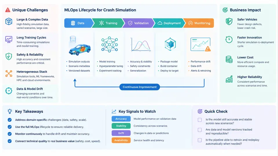
Crash simulation sits at the intersection of high-fidelity physics, regulatory compliance, and expensive hardware testing. A single full-vehicle frontal impact model can contain 8–15 million finite elements, run for 12–36 hours on 64–256 CPU cores, and produce hundreds of gigabytes of d3plot and time-history output. When machine learning enters this workflow — for surrogate modeling, intrusion prediction, material parameter calibration, or design-space exploration — the operational discipline required is fundamentally different from training a model on a static tabular dataset. This chapter establishes why crash-simulation MLOps is its own engineering problem, how the lifecycle differs from generic MLOps, and where the business value actually accumulates.
Why Crash Simulation Breaks Conventional MLOps Assumptions
Generic MLOps pipelines assume that data is cheap to collect, that retraining is a matter of re-reading a data lake, and that model behavior is validated against a held-out sample. Crash simulation violates all three assumptions.
- Data generation is the bottleneck, not training. Each labeled sample is the output of an LS-DYNA, PAM-CRASH, or Radioss run. Generating 2,000 training samples for a surrogate may consume 40,000–200,000 core-hours. The MLOps system must therefore treat simulation jobs as first-class, versioned, and cacheable artifacts — not as an external preprocessing step.
- Physics consistency is a hard constraint. A model that predicts peak intrusion with 3% mean error but violates momentum conservation or produces non-monotonic force-displacement curves is unusable, regardless of its aggregate metric. Validation must include physics-based checks, not only RMSE or R².
- Regulatory traceability is mandatory. FMVSS 208, Euro NCAP, and GB 11551 require that any predictive tool influencing a design decision be traceable to a specific model version, a specific solver version, and a specific set of validated load cases. Reproducibility is a legal requirement, not a best practice.
- Design variables are coupled and constrained. Gauge, material grade, and geometry interact non-linearly. A surrogate trained on a narrow sampling region will silently extrapolate and produce plausible but wrong predictions — a failure mode that is far more dangerous than an obvious crash.
The Crash-Simulation MLOps Lifecycle
The lifecycle below is not a generic ML loop with simulation bolted on. Each stage has crash-specific artifacts and gates.
1. Problem framing and surrogate scope. Define the target quantity (e.g., B-pillar maximum intrusion in mm), the design variables and their bounds, and the load cases in scope. This produces a simulation campaign specification — a versioned document that fixes the DOE, the solver deck template, and the acceptance thresholds before any run is launched.
2. DOE and simulation campaign execution. A typical campaign uses a space-filling design such as Latin Hypercube or a maximin design with 500–3,000 points. Each point is materialized as a parameterized keyword deck, submitted to the HPC scheduler, and tracked by a campaign ID. The MLOps layer must record solver version, element formulation, hourglass control, and mass scaling for every run.
3. Data extraction and feature engineering. Raw d3plot output is reduced to scalar or low-dimensional features: peak force, intrusion at specified nodes, energy absorption, and curve descriptors. This reduction step is itself a versioned transformation, because changing the extraction window or filter changes the training distribution.
4. Model training and physics-aware validation. Training is comparatively cheap. The expensive part is validation: hold-out load cases, extrapolation probes, monotonicity checks, and comparison against physical test data where available.
5. Deployment and inference integration. The surrogate is exposed either as a batch design-space scanner or as an interactive predictor inside the CAD/CAE loop. Latency requirements differ: a batch scan tolerates minutes, an interactive tool needs sub-second response.
6. Monitoring and drift detection. Input drift is detected by comparing the distribution of incoming design vectors against the training DOE. Output drift is detected by periodically running full-fidelity simulations on a monitoring sample and comparing against surrogate predictions.
Where the Business Impact Comes From
The value of crash-simulation MLOps is not "faster training." It is the ability to make design decisions earlier and with quantified confidence. Three concrete impact channels dominate.
| Impact channel | Mechanism | Typical magnitude (example) |
|---|---|---|
| Reduced physical prototypes | Surrogate-guided design space screening narrows candidates before sled and full-vehicle tests | 2–4 fewer full-vehicle tests per program |
| Shortened CAE iteration loop | Interactive surrogate replaces 12–36 h solver runs during early concept phase | Concept-phase iteration from days to minutes |
| Regulatory defensibility | Full traceability from prediction to solver deck to validation evidence | Avoids re-analysis and submission delays |
These magnitudes are illustrative and depend on program scope, vehicle architecture, and the maturity of the existing CAE process. They should be treated as planning assumptions to be validated against a specific program's baseline, not as guaranteed outcomes.
A Minimal Reproducible Example: Campaign Tracking Record
The following is a concrete, fillable campaign record. It is the smallest unit of traceability that makes a surrogate model auditable. Every simulation run in a campaign should produce one such record.
campaign_id:        FRONTAL_ODB_2025_Q1
surrogate_target:   b_pillar_max_intrusion_mm
design_variables:
  - name: b_pillar_gauge
    bounds: [1.2, 2.0]   # mm
  - name: material_grade
    levels: [DP590, DP780, DP980]
  - name: bead_depth
    bounds: [0.0, 8.0]   # mm
doe_method:         maximin_lhs
n_samples:          1200
solver:             LS-DYNA R13.1.0
load_case:          FMVSS208_ODB_64kmh
deck_template:      git://cae/decks/frontal_odb_v7.k
extraction_config:  git://cae/extract/intrusion_v3.yaml
acceptance:
  rmse_max_mm:      4.0
  monotonicity:     required
  ood_load_cases:   [25pct_odb_64kmh, full_frontal_50kmh]
When a model is trained against this campaign, the training script reads the campaign record, resolves the deck and extraction configs by their version-controlled paths, and writes a validation report that references the same campaign ID. If a reviewer later asks "which solver version produced the training data for model v2.3?", the answer is a single lookup, not an archaeology project.
What Makes This Different from Generic MLOps
In a typical ML deployment, the pipeline is: collect data → train → evaluate → deploy → monitor. In crash-simulation MLOps, the pipeline is: specify a campaign → generate expensive labeled data → extract physics-relevant features → train and validate against physics and OOD cases → deploy with traceability → monitor drift and feed back into the campaign. The feedback loops are not optional refinements; they are the mechanism by which the surrogate stays valid as the design space evolves.
The practical consequence is that the MLOps engineer on a crash program must understand solver decks, hourglass energy, and regulatory load cases — not just Docker and Kubernetes. The tooling is necessary but not sufficient. The domain knowledge is what determines whether the system produces trustworthy predictions or expensive noise.