3. Model representation and discretization

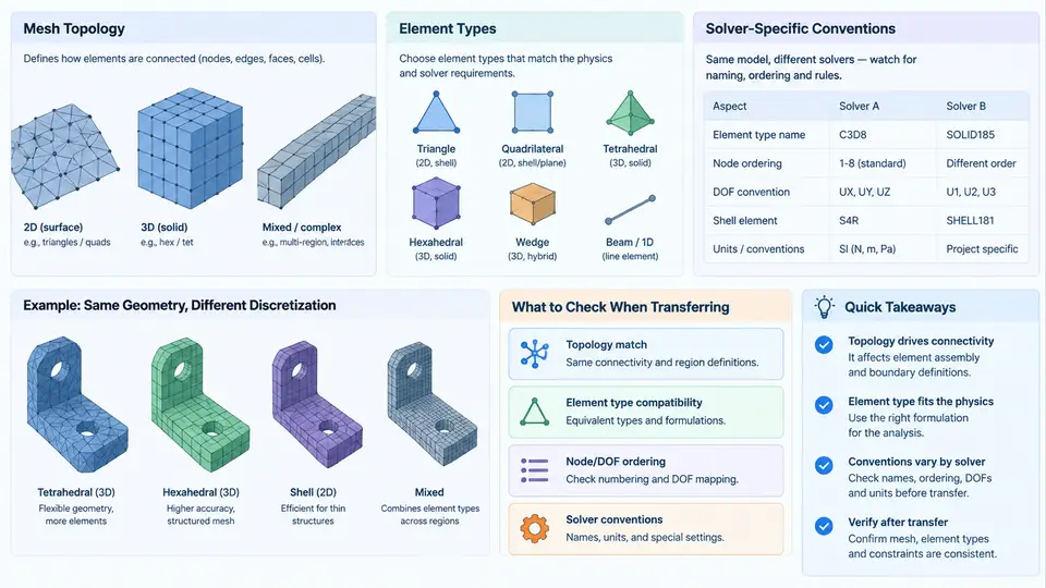
When a CAE model is transferred from one solver to another, the geometry is rarely the problem. The real friction lives in the discretized representation: how the mesh is connected, which element formulations are used, and how each solver interprets the same nominal element. Two models can share identical node coordinates and still produce different stiffness matrices, different mass distributions, and different stress recovery because their topology and element conventions diverge. This chapter examines the three layers that determine whether a transferred model remains physically equivalent: mesh topology, element type mapping, and solver-specific discretization conventions.

Mesh Topology as a Transferable Object

Mesh topology describes the connectivity graph: which nodes belong to which elements, how elements share edges and faces, and whether the resulting assembly is conforming. During transfer, topology is the first thing to verify because it is independent of material and boundary conditions. A topology mismatch will corrupt every downstream result regardless of how carefully loads are mapped.

Consider a simple shell-to-solid transition. In a shell mesh, a stiffener may be represented by offset shell elements sharing nodes with the panel. In a solid mesh, the same stiffener becomes a set of hexahedral or tetrahedral elements whose nodes lie on the panel surface but do not coincide with the shell nodes. If the transfer tool simply writes node coordinates without rebuilding connectivity, the two regions become mechanically disconnected. The model solves, but the stiffener carries no load. This is a classic silent failure in cross-solver transfer.

Topology checks should therefore precede any solver run. The essential checks are: free or unconnected nodes, duplicate nodes within a tolerance, non-manifold edges where more than two elements share an edge, and inverted or zero-area elements. A practical tolerance for duplicate node detection is typically 1e-4 to 1e-3 of the model's characteristic length, but this must be stated explicitly because different solvers use different default merge tolerances.

Element Types and Formulation Mapping

Element type names are not portable. A C3D8 in Abaqus, a SOLID185 in ANSYS, and a CHEXA in Nastran may all describe an eight-node hexahedron, but their formulations differ in integration scheme, hourglass control, and shear locking treatment. Transferring a model means mapping not just the element shape but the formulation intent.

The critical distinctions are:

• Integration order: Full integration versus reduced integration. A reduced-integration hex with hourglass control behaves very differently from a fully integrated hex under bending. If the target solver lacks an equivalent hourglass stabilization, the transferred element may be too stiff or exhibit spurious modes.
• Element family: First-order (linear) versus second-order (quadratic). Second-order tets are often preferred for stress accuracy, but they are more sensitive to distorted geometry and can produce different contact behavior.
• Shell formulation: Thin shell, thick shell, and continuum shell are not interchangeable. Transferring a thin-shell model into a continuum-shell formulation changes transverse shear behavior and through-thickness stress distribution.
• Beam and truss: Section integration, offset, and end-release definitions must be mapped explicitly. A beam transferred without its offset will shift the neutral axis and change bending stiffness.

A useful practice is to build an element mapping table before transfer. The table records the source element type, the intended formulation, the target element type, and any compensating settings. This table becomes part of the transferability evidence package.

Source element	Formulation intent	Target element	Compensation required
C3D8R (reduced hex)	Efficient solid, bending dominant	SOLID185 with reduced integration	Enable hourglass control; verify stiffness
S4R (shell)	Thin shell, membrane + bending	SHELL181	Check section offset and shear correction
B31 (beam)	Timoshenko beam with offset	BEAM188	Re-enter section offset and end releases
C3D10 (quadratic tet)	Stress accuracy in complex geometry	SOLID187	Verify midside node placement and Jacobian

Solver-Specific Conventions That Break Equivalence

Even with correct topology and element mapping, solver conventions can introduce systematic differences. These conventions are not bugs; they are documented behaviors that must be accounted for during transfer.

Node and element numbering. Most solvers renumber internally, but user-defined sets, surfaces, and contact pairs reference original IDs. If the transfer tool renumbers without updating references, boundary conditions may attach to the wrong entities. Always export and re-import named selections explicitly.

Coordinate systems. Material orientations, beam sections, and shell normals depend on local coordinate systems. A shell normal that points in the opposite direction after transfer will reverse the sign of bending stresses. The convention for defining shell normals (node ordering, right-hand rule) must be checked in both solvers.

Degrees of freedom. Shell and beam elements carry rotational DOFs; solid elements do not. When a shell region is transferred to solids, rotational loads and constraints must be converted to equivalent nodal forces or kinematic couplings. Ignoring this produces either a singular stiffness matrix or an over-constrained model.

Units and consistent scaling. Some solvers are unit-agnostic, others assume consistent unit systems. A model transferred in millimeters and tonnes will produce stresses in MPa only if the density and modulus are scaled consistently. Unit inconsistency is one of the most common causes of apparently nonsensical transfer results.

Practical Transfer Example: Shell-Stiffened Panel

To make the process concrete, consider a stiffened panel modeled in Solver A with S4R shells for the skin and B31 beams for the stiffeners, then transferred to Solver B using SHELL181 and BEAM188. The transfer proceeds as follows.

Inputs: The source model has 12,400 shell elements, 860 beam elements, and 14,200 nodes. The skin is 2.0 mm thick aluminum (E = 70 GPa, ν = 0.33, ρ = 2.7e-9 tonne/mm³). Stiffeners are 50 × 3 mm rectangular sections offset 25 mm from the skin mid-surface. A 1.0 MPa pressure load acts on the skin, and the panel is clamped along two opposite edges.

Transfer steps:

1. Export the mesh in a neutral format (e.g., Nastran bulk data or a solver-neutral mesh file) with nodes, elements, and named sets.
2. Import into Solver B and run a topology check. In this example, the import reveals 38 duplicate nodes along the stiffener-skin interface caused by a tolerance mismatch. Merging them at 0.01 mm restores connectivity.
3. Map element types. S4R → SHELL181 with reduced integration and hourglass control. B31 → BEAM188 with the same rectangular section and a 25 mm offset. The offset must be re-entered because Solver B does not read Solver A's offset definition directly.
4. Reapply boundary conditions. The clamped edges are defined as node sets; verify that the set membership survived renumbering. In this example, 12 nodes on one edge were lost because the original set referenced a geometric edge that no longer exists after import. Re-select them by coordinate box.
5. Apply the pressure load. Confirm that the shell normal direction is consistent. If normals are flipped, the pressure acts in the opposite direction and the panel deflects the wrong way.

Observable verification: After solving, compare the first natural frequency and the maximum deflection at the panel center against the source model. A reasonable acceptance band for a well-transferred model is within 2–5% for frequency and 5% for deflection, assuming identical material and boundary conditions. Larger deviations point to a specific layer: a frequency shift with unchanged static deflection often indicates a mass or offset error; a deflection change with unchanged frequency suggests a stiffness or boundary condition error.

Building a Transferable Discretization Record

The most reliable way to manage these issues is to treat the discretization as a documented artifact. For each transfer, record the source and target element types, the formulation intent, the integration scheme, the offset and section definitions, the merge tolerance used, and the verification metrics. This record turns a one-off transfer into a repeatable process and provides the evidence needed when results are questioned.

A minimal record for the stiffened panel example would include: source solver and version, target solver and version, element mapping table, node merge tolerance (0.01 mm), boundary condition set reconstruction method, and the frequency and deflection comparison with percentage deviation. When the same model is transferred again—for a design iteration or a different load case—this record becomes the baseline for detecting new discrepancies.

Discretization transfer is not a file conversion problem. It is a modeling equivalence problem. The mesh topology, element formulations, and solver conventions each carry physical meaning, and preserving that meaning requires explicit verification at every layer. A model that solves is not necessarily a model that transferred correctly; only a model that reproduces the intended physics can be trusted for cross-solver assessment.