1. Cross-solver CAE data landscape
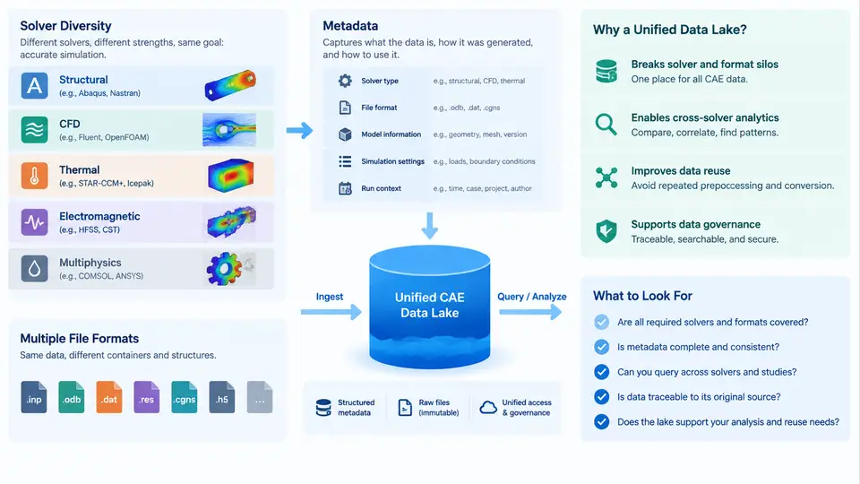
Any organization running more than one simulation tool eventually hits the same wall: the results exist, but they cannot be compared, searched, or reused at scale. A crash analyst has LS-DYNA d3plot output; a thermal engineer has ANSYS .rst files; an aerodynamics team has SU2 or Fluent case/data pairs; a structures group has Nastran .op2 and Abaqus .odb. Each format is internally consistent, each solver is validated, and yet the aggregate engineering knowledge of the company is effectively locked inside a few hundred thousand files scattered across project shares, HPC scratch directories, and personal workstations. This chapter maps that landscape and explains why a unified CAE data lake is the natural architectural response.
Why Solver Diversity Is Structural, Not Accidental
Solver diversity is not a symptom of poor standardization. It is a direct consequence of physics specialization. Explicit dynamics codes such as LS-DYNA and Radioss are built around small, stable time steps and contact-dominated workloads; implicit structural codes such as Abaqus/Standard and Nastran solve large sparse systems where convergence behavior dominates runtime; CFD codes such as Fluent, STAR-CCM+, and OpenFOAM operate on unstructured polyhedral meshes with field variables defined per cell and per face; electromagnetic and multiphysics tools add yet another discretization philosophy. Each solver therefore defines its own element library, its own result quantities, its own time/iteration semantics, and its own file layout.
The practical consequence is that a single vehicle program may legitimately produce dozens of distinct result formats for one physical event. A frontal crash model, for example, might generate:
- LS-DYNA
d3plot/binoutfor transient structural response, - PAM-CRASH or Radioss result files for a supplier-owned subsystem,
- Nastran
.op2for the body-in-white modal check, - Fluent
.cas/.datfor occupant thermal comfort, - CSV exports from a Python post-processing script for KPI dashboards.
None of these can be opened by the others' native tools. Cross-solver comparison today is usually done by exporting everything to CSV or by manually re-running cases in a common tool — both approaches destroy fidelity and provenance.
File Formats: A Three-Layer Taxonomy
To design a data lake, it helps to classify CAE files by role rather than by vendor. Three layers matter:
| Layer | Typical artifacts | Characteristics |
|---|---|---|
| Model / input | .key, .inp, .bdf, .cas, .jou |
Text or mixed; defines mesh, materials, BCs, solver controls; version-sensitive |
| Result / binary | d3plot, .odb, .op2, .rst, .dat |
Binary, solver-specific, often hundreds of GB; contains time-history and field data |
| Derived / exchange | CSV, HDF5, VTK/VTU, EnSight .case, JSON KPI files |
Post-processed, tool-neutral, suitable for analytics but lossy relative to native results |
The key insight for lake design: native binaries should be stored as immutable objects, while derived formats are what analytics actually queries. Trying to parse d3plot on every dashboard request is not viable; extracting a curated HDF5 or Parquet layer once per run is.
Metadata: The Real Differentiator
File formats are a storage problem; metadata is a discovery problem. A CAE data lake lives or dies on the quality of its metadata model. At minimum, each simulation artifact should carry:
- Identity: run ID, solver name and version, license feature used, host, user, timestamp.
- Model context: project, vehicle or product variant, subsystem, mesh size (nodes/elements), unit system.
- Physics context: analysis type (crash, NVH, CFD steady, thermal transient), load case ID, boundary condition summary.
- Provenance: parent run ID, input deck hash, git commit of the automation script, solver command line.
- Outcome: exit status, wall-clock time, convergence flag, extracted KPIs (e.g., peak acceleration, max von Mises stress, drag coefficient).
In practice, most of this metadata is not written by the solver. It must be captured by the job submission wrapper, the post-processing script, or a dedicated ingestion agent. This is the single most underestimated engineering effort in CAE data lake projects.
From File Shares to a Unified Data Lake
The motivation for a unified lake becomes clear when you compare the current state with the target state. Today, finding "all frontal crash runs of the B-pillar for variant X in the last 18 months" requires tribal knowledge, filesystem archaeology, and often a phone call. In a lake, the same query is a metadata filter followed by a columnar scan over extracted KPIs.
The architecture that makes this work separates four concerns:
- Object storage for raw native files, addressed by content hash and run ID.
- Metadata catalog (relational or graph) holding the fields listed above, indexed for search.
- Extraction layer that converts native results into analytics-friendly formats (HDF5 for fields, Parquet for time series and KPIs).
- Query and visualization layer that never touches native binaries directly.
What "Unified" Actually Requires
A common misconception is that unification means converting everything to one format. That is neither feasible nor desirable — no single format preserves the semantics of explicit crash, implicit modal, and steady CFD results simultaneously. Unification instead means three concrete capabilities:
- Unified addressing. Every artifact, regardless of solver, is reachable through one identifier scheme (e.g.,
run://project/variant/loadcase/run-id). - Unified metadata schema. A common set of fields with solver-specific extensions, so that a query can span LS-DYNA and Abaqus runs without special-casing.
- Unified access pattern. Analysts and scripts use the same API to retrieve KPIs, time histories, or field snapshots, whether the underlying source was
d3plotor.odb.
A Minimal Reproducible Example
Consider a small but realistic ingestion scenario. A crash run produces d3plot output, and the job wrapper writes a sidecar JSON alongside it:
{
  "run_id": "CR-2024-0417-BPILLAR-V3",
  "solver": "ls-dyna",
  "solver_version": "R13.1",
  "analysis_type": "frontal_crash",
  "load_case": "NCAP-FR-56kph",
  "variant": "B-pillar-V3",
  "mesh": { "nodes": 2843117, "elements": 2760442 },
  "units": "mm-ton-s",
  "input_deck_sha256": "a3f1...9c2e",
  "artifacts": ["d3plot", "binout", "glstat"],
  "kpis": {
    "peak_intrusion_mm": 142.7,
    "peak_accel_g": 48.3,
    "mass_kg": 1.42
  },
  "status": "completed",
  "wall_clock_s": 18740
}
The ingestion agent then: (1) uploads the native files to object storage keyed by run_id; (2) inserts the metadata row into the catalog; (3) runs a parser that extracts the intrusion time history into a Parquet file partitioned by variant and load_case. A verification step confirms that the KPI values in the sidecar match those recomputed from the parsed time history within a tolerance (e.g., 0.5%). If they diverge, the run is flagged rather than silently accepted — a common failure mode when solver versions change output conventions.
Typical failure symptoms at this stage include missing sidecar files (wrapper not invoked), unit mismatches (mm-ton-s vs. m-kg-s producing KPIs off by orders of magnitude), and parser version drift after a solver upgrade. Each of these should be detectable from the catalog itself, which is precisely why metadata completeness matters more than storage volume in the early phases of a lake project.
Scope of This Course
The remaining chapters build on this landscape: metadata schema design, ingestion pipeline engineering, format conversion and validation, cross-solver KPI normalization, query patterns, and analytics workflows such as surrogate modeling and design-space exploration. The recurring theme is that solver diversity is a given — the engineering task is to make that diversity queryable without flattening it.