3. Common anomalies in crash CAE datasets
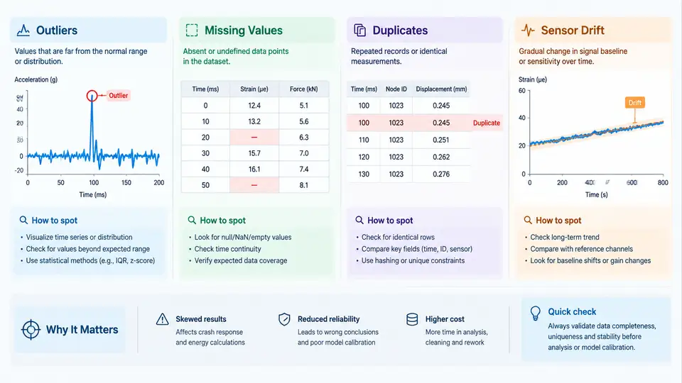
Crash CAE datasets are assembled from many sources: full-vehicle explicit dynamics runs, sled tests, component-level simulations, physical crash tests, and post-processing pipelines that extract hundreds of channels per event. Before any anomaly detection model can be trusted, the raw dataset itself must be characterized. Four anomaly families dominate crash CAE data quality work: outliers, missing values, duplicates, and sensor drift. Each has a distinct physical or procedural origin, a distinct statistical signature, and a distinct remediation path. Treating them as one generic "dirty data" problem is the most common mistake in early-stage data quality projects.
Outliers: extreme values with physical or numerical causes
In crash CAE, an outlier is a sample that deviates so far from the expected response that it cannot be explained by normal run-to-run variation. Typical channels include acceleration_X, acceleration_Y, acceleration_Z, intrusion, force, and energy_absorbed. Outliers arise from at least four mechanisms:
- Numerical instability — hourglassing in under-integrated solid elements, negative volume errors in highly distorted elements, or contact penetration producing spurious spikes.
- Unit and scaling errors — a channel recorded in
gmixed with one recorded inm/s², or a force channel inNmixed withkN. - Sensor saturation or clipping — a physical accelerometer exceeding its rated range, producing a flat-topped plateau rather than a true peak.
- Genuine physical events — a real severe impact that is statistically extreme but valid.
The practical difficulty is that the fourth category must be preserved. A robust screening approach combines a global statistical test with a local physical plausibility check. For example, compute the modified Z-score using median absolute deviation (MAD):
MAD = median(|x_i - median(x)|)
M_i = 0.6745 * (x_i - median(x)) / MAD
flag if |M_i| > 3.5
A sample flagged by MAD is then cross-checked against the physical envelope: does the peak acceleration exceed the sensor's rated range? Does the intrusion time history show a discontinuity consistent with element deletion? Only samples that fail both the statistical and the physical test should be marked as true outliers. This two-stage logic prevents the common error of discarding legitimate high-severity crash pulses.
Missing values: structural gaps, not random noise
Missing data in crash CAE is rarely missing completely at random. It is usually structural: a channel was not requested in the output deck, a sensor failed during the test, a simulation terminated early due to negative volume, or a post-processing script skipped a run because the d3plot file was incomplete. The missingness pattern itself carries information.
Three patterns are worth distinguishing:
- Channel-level missingness — an entire channel is absent for a subset of runs. This often correlates with a specific solver version, output request, or test setup.
- Time-window missingness — a channel exists but has gaps in specific time intervals, typical of sensor dropout or data acquisition buffer overflow.
- Run-level missingness — an entire run is absent, usually due to solver divergence or test cancellation.
Imputation should be chosen according to the pattern. For channel-level missingness, mean or median imputation is usually acceptable if the missing fraction is below roughly 5% and the channel is not a primary injury metric. For time-window gaps in a time-history channel, linear interpolation is often adequate for smooth channels such as intrusion, but is dangerous for oscillatory channels such as acceleration, where interpolation can artificially reduce peak values. In that case, flag the run for review rather than imputing. Run-level missingness should generally not be imputed at all; it should be recorded as a separate quality flag so that downstream models can exclude or weight those runs explicitly.
Duplicates: exact, near, and semantic
Duplicates in crash CAE datasets appear in three forms. Exact duplicates are identical rows, usually caused by a re-run of an extraction script or a database join that multiplied records. Near duplicates are runs that differ only in metadata such as run_id or timestamp but share identical physical inputs and outputs. Semantic duplicates are runs with different IDs but effectively the same configuration — for example, the same sled test repeated on different days with the same pulse and the same dummy.
Detection strategy depends on the form. Exact duplicates are removed by hashing the full feature vector. Near duplicates require a key-based comparison: define a composite key from the physical configuration columns (vehicle model, impact speed, impact angle, barrier type, dummy type) and check for collisions. Semantic duplicates require domain judgment and are best handled by clustering on the input parameter space and reviewing cluster members manually.
The risk of leaving duplicates in place is severe for anomaly detection: a duplicated run effectively doubles its weight in distance-based or density-based models, biasing the learned normal region and masking true anomalies.
Sensor drift: slow, systematic deviation over time
Sensor drift is a gradual change in a channel's baseline or sensitivity across a sequence of tests or simulation batches. In physical crash testing, drift commonly appears in accelerometers and load cells due to thermal effects, mounting degradation, or amplifier aging. In CAE, an analogous drift can appear when a solver version, contact parameter, or material card is updated mid-campaign, producing a slow shift in response that is not caused by any physical change in the test article.
Drift is the hardest anomaly to detect because each individual run may look normal. The signature is a trend in a derived statistic — for example, the pre-impact baseline of acceleration_X, or the ratio of peak force to peak intrusion — plotted against run order or calendar date. A practical detection method is to compute a rolling median of the baseline offset over a window of 20–30 runs and flag runs where the offset exceeds a threshold derived from the sensor's calibration tolerance.
Putting the four families into a single screening workflow
A practical screening pass over a crash CAE dataset can be organized as a short sequence of checks, each producing a quality flag rather than a silent modification. The following example uses a tabular dataset with columns run_id, vehicle_model, impact_speed, impact_angle, acceleration_X_peak, intrusion_max, HIC, and run_date.
1. Exact duplicate check
   hash = sha256(run_id + vehicle_model + impact_speed + impact_angle)
   flag_exact_dup = duplicated(hash)

2. Near duplicate check
   key = (vehicle_model, impact_speed, impact_angle, barrier_type)
   flag_near_dup = duplicated(key) & ~flag_exact_dup

3. Missing value audit
   for each channel:
       missing_rate = count(null) / count(*)
       if missing_rate > 0.05: flag_channel_missing
       if channel is primary injury metric and missing_rate > 0: flag_primary_missing

4. Outlier screening
   M = 0.6745 * (x - median(x)) / MAD(x)
   flag_stat_outlier = abs(M) > 3.5
   flag_phys_outlier = acceleration_X_peak > sensor_rated_range
   flag_true_outlier = flag_stat_outlier & flag_phys_outlier

5. Drift screening
   baseline = rolling_median(acceleration_X_baseline, window=25)
   flag_drift = abs(baseline - calibration_reference) > tolerance
The output of this pass is not a cleaned dataset but an annotated one. Each row carries boolean flags, and each flag has a documented meaning. Downstream anomaly detection models can then choose to exclude flagged rows, weight them, or treat the flags themselves as features. This separation between detection and remediation is what makes the pipeline auditable.
flag_true_outlier exceeds roughly 2–3% of runs, the threshold is probably too aggressive or the physical envelope is misconfigured. If flag_drift is zero across a long campaign, the drift window or tolerance is likely too wide to detect anything.Why these four families matter for anomaly detection
Outliers, missing values, duplicates, and sensor drift are not merely preprocessing nuisances. Each one distorts the statistical geometry that anomaly detection algorithms rely on. Outliers inflate variance and pull decision boundaries. Missing values reduce effective sample size and can introduce bias if missingness correlates with the target. Duplicates artificially densify certain regions of feature space. Drift shifts the baseline over time, so a model trained on early runs will systematically misclassify later ones. Recognizing these four families, understanding their crash-CAE-specific origins, and applying targeted detection rather than generic cleaning is the foundation for every subsequent chapter in this course.