3. AI/ML requirements for CAE datasets
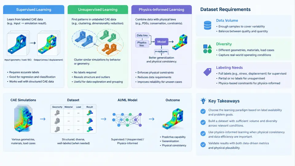
CAE simulation datasets are not generic tabular collections. They are structured, physics-constrained, multi-field records whose usefulness depends entirely on the learning paradigm they are meant to serve. A dataset that trains a surrogate for steady-state CFD is fundamentally different from one that trains a physics-informed neural network (PINN) to solve a parametric PDE, or one that clusters crash topologies without any labels at all. This section maps the three dominant learning paradigms onto their concrete dataset requirements, then quantifies the volume, diversity, and labeling decisions that follow.
Supervised Learning: Input–Output Pairs with Physical Fidelity
Supervised learning dominates CAE surrogate modeling. The dataset is a set of paired samples (x, y), where x encodes design or boundary parameters and y is the simulated field response. Typical x vectors include geometry parameters (chord length, fillet radius, thickness), boundary conditions (inlet velocity, wall temperature), and material properties (Young's modulus, density). Typical y fields include pressure, velocity, von Mises stress, or temperature distributions sampled on a mesh.
The critical requirement is consistency of the discretization. If sample A stores pressure on a 120k-cell mesh and sample B on an 80k-cell mesh, a naive CNN or GNN cannot batch them. Two practical solutions exist: (1) remap all fields to a common reference mesh via interpolation, or (2) store fields on a fixed-resolution voxel or image grid. The second option is common for CNN surrogates; the first is preferred for graph neural networks operating on native meshes.
For a concrete example, consider a 2D airfoil lift surrogate. Inputs: angle of attack α ∈ [−4°, 16°], Reynolds number Re ∈ [1×10⁶, 5×10⁶], and NACA thickness ratio t/c ∈ [0.08, 0.16]. Outputs: lift coefficient CL and pressure field on a 256×256 Cartesian grid. A Latin hypercube sample of 500 cases, each solved with a RANS solver, yields a dataset of 500 paired samples. Splitting 80/10/10 for train/validation/test, a CNN typically reaches R² > 0.97 on CL with 400 training samples — but only if the pressure fields are normalized per-sample (zero-mean, unit-variance) before training.
Unsupervised Learning: Structure Discovery Without Labels
Unsupervised methods — autoencoders, PCA, clustering, and self-supervised pretraining — require no y labels but demand broad coverage of the input space. Their purpose is dimensionality reduction, anomaly detection, or feature extraction for downstream tasks. A convolutional autoencoder trained on 5,000 CFD snapshots can compress a 256×256 field into a 32-dimensional latent vector while preserving 99% of variance; that latent space then supports clustering of flow regimes or fast similarity search.
The dataset requirement here is diversity, not labeling. If all 5,000 snapshots come from a single operating point, the latent space collapses and the autoencoder learns nothing generalizable. A practical rule: sample the parameter space so that no single regime occupies more than 30% of the dataset. For a heat-exchanger study, that means balancing laminar, transitional, and turbulent cases rather than letting the solver's default regime dominate.
Physics-Informed Learning: Residuals, Not Just Labels
Physics-informed neural networks (PINNs) and physics-informed surrogates embed governing equations — Navier–Stokes, elasticity, heat conduction — directly into the loss function. The dataset requirement shifts: instead of dense labeled fields, PINNs need collocation points (where PDE residuals are evaluated), boundary/initial condition points, and optionally a small set of labeled observations for data assimilation.
A PINN for 2D steady heat conduction on a square domain might use 10,000 interior collocation points, 400 boundary points, and 50 sparse temperature measurements. The loss combines the PDE residual, boundary mismatch, and data mismatch:
L = λ_pde · mean(∇²T)² + λ_bc · mean(T_boundary − T_bc)² + λ_data · mean(T_obs − T_measured)²Here the dataset is not a table of input–output pairs but a point cloud with role tags: each point is labeled as interior, boundary, or observation. This is a fundamentally different data schema, and mixing it with supervised datasets without explicit role metadata causes silent training failures.
Data Volume: How Much Is Enough?
Volume requirements scale with input dimensionality and output complexity. For low-dimensional regression (e.g., predicting drag from 5 shape parameters), 200–500 samples often suffice. For field prediction on a 256×256 grid, expect 1,000–10,000 samples. For 3D transient fields, 10,000+ samples are common. These are empirical ranges, not guarantees — the actual requirement depends on the intrinsic dimensionality of the solution manifold.
A practical diagnostic: train the surrogate on increasing subsets (100, 200, 500, 1000 samples) and plot validation error. If the error curve has flattened, adding more samples of the same kind yields diminishing returns; the bottleneck is diversity, not volume. If the curve is still descending steeply, collect more data within the existing parameter ranges.
Diversity: The Hidden Requirement
Diversity operates along three axes: geometric (shape variation), operational (boundary conditions, Reynolds number, load cases), and numerical (mesh resolution, solver settings, turbulence models). A dataset that varies geometry but fixes the turbulence model will produce a surrogate that fails when the model changes. Document the diversity axes explicitly in the dataset metadata — this is as important as the raw sample count.
Labeling Needs and Cost Trade-offs
In CAE, labels are simulation outputs, so labeling cost equals solver cost. A single high-fidelity CFD run may take hours to days. This makes active learning attractive: train an initial surrogate on 100 samples, then query the solver only for samples where the surrogate's predicted uncertainty is highest. This can reduce solver calls by 40–60% compared to random sampling while achieving comparable accuracy.
| Paradigm | Typical Sample Count | Label Source | Key Risk |
|---|---|---|---|
| Supervised | 10²–10⁴ | Solver output fields | Mesh inconsistency across samples |
| Unsupervised | 10³–10⁵ | None | Narrow parameter coverage |
| Physics-informed | 10³–10⁵ collocation points | Sparse observations + PDE | Loss balancing (λ weights) |
The dataset engineer's job is to translate the intended learning paradigm into a concrete schema, sampling plan, and labeling budget before any solver time is spent. Getting this wrong at the dataset stage is expensive to fix later — retraining a surrogate is cheap; re-running 5,000 CFD cases is not.