1. CAE simulation dataset engineering for A
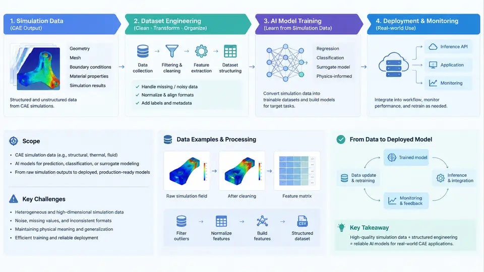
CAE simulation dataset engineering is the discipline of turning solver-generated physics data into training-ready assets for machine learning models. It sits between two mature worlds — numerical simulation and machine learning — and inherits constraints from both. A CFD engineer cares about mesh quality, turbulence model selection, and convergence residuals. An ML engineer cares about sample distribution, label noise, and train/validation leakage. Dataset engineering must satisfy both simultaneously, and that dual obligation is what makes the field genuinely difficult rather than merely tedious.
What Falls Inside the Scope
The scope is broader than "running simulations and saving results." A working definition covers five connected responsibilities:
- Problem formalization. Translating an engineering question into a learnable mapping — for example, "predict drag coefficient from geometry" becomes a regression task with a defined input tensor (voxelized or point-cloud geometry) and a scalar target.
- Design space definition. Specifying which parameters vary, over what ranges, and with what sampling strategy. This determines whether the dataset covers the operating envelope the deployed model will actually see.
- Simulation campaign execution. Automating mesh generation, solver setup, job submission, and failure recovery across hundreds or thousands of cases.
- Data extraction and transformation. Converting native solver output (CGNS, EnSight, VTK, HDF5) into tensors, with consistent normalization and coordinate conventions.
- Dataset versioning and governance. Tracking which cases belong to which split, which solver version produced them, and which preprocessing revision was applied.
A useful mental model is that the dataset is a product with its own specification, not a byproduct of simulation runs. Once that framing is adopted, questions like "what is the acceptance criterion for a case?" and "how do we handle a partially converged run?" become design decisions rather than afterthoughts.
Why This Is Hard: Four Structural Challenges
Cost asymmetry. A single high-fidelity transient CFD case may consume 500–5,000 core-hours. Generating 10,000 samples is therefore a budget problem, not just a compute problem. This forces deliberate sampling — Latin hypercube, Sobol sequences, or adaptive design of experiments — rather than uniform grids.
Distribution shift between training and deployment. Training samples are typically drawn from a parametric design space. Deployed models encounter real geometries with manufacturing tolerances, sensor noise, and operating conditions outside the sampled envelope. A model that achieves 2% mean absolute error on the test split can fail catastrophically on an out-of-distribution inlet profile.
Label quality is not binary. Unlike image classification, simulation outputs have continuous quality. A case may be converged to 1e-4 residuals, or 1e-3, or may have stalled. Mixing these into one dataset without quality flags injects systematic error that no amount of model capacity can correct.
Reproducibility across toolchains. Solver version, turbulence closure, mesh topology, and even compiler flags affect results. A dataset assembled over eighteen months may contain data from three solver releases. Without metadata capture, the model learns a mixture of physics and software-version artifacts.
The End-to-End Workflow
The workflow below is the backbone of this course. Each stage produces artifacts that the next stage consumes, and each has its own failure modes.
Two features of this diagram deserve emphasis. First, the feedback loop from evaluation back to sampling is not optional. In practice, the first training run almost always reveals coverage gaps — regions of the design space where the model performs poorly because too few samples exist there. Adaptive resampling, guided by model error, is the standard remedy. Second, the metadata band runs underneath every stage. Solver version, mesh statistics, convergence residuals, and preprocessing revision must be captured at the moment of generation, because reconstructing them later is often impossible.
A Concrete Illustration: Airfoil Drag Prediction
Consider a representative task: predict the drag coefficient Cd of a 2D airfoil from its shape and operating condition. The input is a parameterized geometry (e.g., CST or B-spline control points) plus angle of attack and Reynolds number. The target is Cd from a RANS solve.
A defensible dataset specification might look like this:
| Field | Example value / range | Notes |
|---|---|---|
| Geometry parameterization | 8 CST weights, upper + lower | Bounds enforce non-self-intersecting profiles |
| Angle of attack | −4° to 14°, 1° step | Beyond 14° flow separation dominates |
| Reynolds number | 1e6, 3e6, 5e6 | Three discrete levels |
| Mesh | ~80k cells, y+ < 1 | Same topology family for all cases |
| Solver | SU2 7.5.1, SST k-ω | Version pinned in metadata |
| Convergence criterion | RMS residual < 1e-5 | Cases failing this are flagged, not discarded |
| Sampling | Latin hypercube, 2,000 cases | Plus 200 boundary cases |
With 2,000 cases at roughly 30 minutes each on 16 cores, the campaign consumes about 16,000 core-hours — a realistic but non-trivial budget. The boundary cases (near stall, extreme thickness) are deliberately over-represented because they are where models most often fail.
After simulation, extraction converts each case into a fixed-size tensor: geometry sampled on a 128-point surface grid, plus two scalar conditions. The target is a single scalar. Splits are assigned by geometry cluster, not randomly, to prevent near-duplicate shapes from appearing in both training and test sets — a subtle leakage source that inflates reported accuracy.
What Separates a Working Dataset from a Failed One
Three practices consistently distinguish successful projects. First, quality flags instead of silent filtering: a case that converged to 1e-4 is still useful for pretraining or as a low-confidence sample, but only if that status is recorded. Second, split assignment before any preprocessing: normalization statistics computed on the full dataset leak test information into training. Third, an out-of-distribution holdout: a set of geometries or operating conditions deliberately excluded from the design space, used to estimate how the model behaves when it encounters something genuinely new.
The remaining chapters of this course expand each stage of this workflow: sampling strategies and their statistical properties, solver automation and failure handling, format conversion and tensor design, split methodology, uncertainty-aware labeling, and deployment monitoring. The through-line is consistent — every decision in dataset engineering is ultimately a decision about what the model will and will not be able to learn.