1. Automotive CAE data landscape

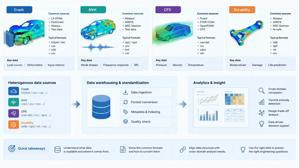
Automotive CAE is not a single simulation discipline; it is a federation of physics domains, each producing data with its own structure, cadence, and analytical intent. Before any warehouse schema or SQL query can be designed, the data engineer must understand what each domain actually emits. This chapter maps the four dominant CAE domains — crash, NVH, CFD, and durability — and establishes the analytical requirements that will drive every downstream modeling decision.

Domain-by-Domain Data Characteristics

Crash simulation (frontal, side, rear, pedestrian protection) is dominated by explicit finite-element solvers such as LS-DYNA, PAM-CRASH, and Radioss. A single full-vehicle frontal impact model may contain 8–15 million elements and run for 100–150 ms of physical time. The solver writes time-history output at fixed intervals — typically every 0.5–1.0 ms — producing nodal displacement, velocity, acceleration, and element stress/strain for selected output blocks. A single run can generate 50–500 GB of raw d3plot and binout files. The analytical questions are event-centric: Did the occupant compartment maintain integrity? What was the peak B-pillar acceleration? Did the airbag trigger within the required window? These are threshold and time-series queries, not spatial averages.

NVH simulation (noise, vibration, harshness) uses implicit solvers — Nastran, OptiStruct, Abaqus — to compute normal modes, frequency response functions, and acoustic cavity modes. A body-in-white modal analysis might extract 200–500 modes in the 0–200 Hz range. The output is fundamentally spectral: eigenfrequencies, mode shapes (large vector files), and transfer functions. Data volume per run is smaller than crash (1–20 GB), but the analytical requirement is different — engineers compare mode frequencies against target bands, check mode shape participation, and correlate with test data. Queries are comparative and statistical across design variants.

CFD simulation (aerodynamics, thermal management, cabin climate) solves the Navier-Stokes equations on meshes of 50–300 million cells. Solvers like Fluent, STAR-CCM+, and PowerFLOW produce field data (pressure, velocity, temperature) at each iteration or time step. A transient external aero run may write 10,000+ field snapshots. The analytical focus is on integrated quantities — drag coefficient (Cd), lift coefficient (Cl), mass flow rates — and on spatial field patterns for flow separation and recirculation. CFD data is the most voluminous per run and the most spatially complex.

Durability simulation (fatigue, static stiffness, thermal cycling) combines implicit FEA with material fatigue models. A full-body fatigue analysis may evaluate 10⁶–10⁸ cycles across 500+ load cases derived from road load data. Output includes damage accumulation, safety factors, and hotspot locations. The analytical requirement is lifecycle-oriented: Which joints fail first? What is the margin to target? How does damage vary across load cases? Data volume is moderate (5–50 GB) but the metadata — load case definitions, material curves, cycle counts — is rich and critical.

Common Metadata and the Case for a Warehouse

Despite their differences, all four domains share a common metadata spine: a simulation case is always defined by a vehicle program, a design variant (e.g., BIW-042), a load case or boundary condition set, a solver version, a mesh iteration, and a run timestamp. This metadata is the join key that makes cross-domain analytics possible. Without it, crash results cannot be correlated with NVH modes on the same design variant, and CFD drag cannot be tracked against durability load cases across a program timeline.

The practical problem is that this metadata lives in different places: solver deck headers, directory naming conventions, PLM systems, and engineer spreadsheets. A CAE data warehouse exists to extract, normalize, and persist this metadata alongside the numerical results, so that SQL can answer questions like: "For program X, show all design variants where the frontal crash peak acceleration exceeded 50 g and the first torsional mode dropped below 32 Hz."

Analytical Requirements That Shape the Schema

The four domains impose distinct query patterns that a single flat table cannot satisfy efficiently:

• Time-series queries (crash): Need efficient range scans and peak detection over 100–300 time steps per channel. A columnar store or partitioned table by run ID works well.
• Spectral queries (NVH): Need frequency-band filtering and mode matching. Storing eigenfrequencies as indexed scalar values enables fast band queries.
• Spatial field queries (CFD): Need aggregation over mesh regions and comparison of integrated coefficients. Storing derived scalars (Cd, Cl) alongside field metadata avoids scanning raw field files.
• Lifecycle queries (durability): Need load-case ranking and damage accumulation across hundreds of cases. A normalized load-case table with foreign keys to run IDs supports this.

Practical Example: Normalizing a Crash Run into Queryable Rows

Consider a frontal impact run for BIW-042, solver LS-DYNA v13.1, 120 ms physical time, output every 1.0 ms. The binout file contains acceleration at the B-pillar left node (node ID 20451). A typical ETL step extracts this channel and writes rows like:

INSERT INTO cae_time_history (run_id, channel_name, time_ms, value)
VALUES
  ('FR-2024-0042', 'B_PILLAR_L_ACCEL', 0.0,  0.12),
  ('FR-2024-0042', 'B_PILLAR_L_ACCEL', 1.0,  2.45),
  ('FR-2024-0042', 'B_PILLAR_L_ACCEL', 2.0,  8.91),
  ...
  ('FR-2024-0042', 'B_PILLAR_L_ACCEL', 120.0, 0.03);

With this table, a peak-acceleration query is straightforward:

SELECT run_id, MAX(value) AS peak_accel_g
FROM cae_time_history
WHERE channel_name = 'B_PILLAR_L_ACCEL'
  AND run_id IN (SELECT run_id FROM cae_run WHERE program = 'X' AND variant = 'BIW-042')
GROUP BY run_id
HAVING MAX(value) > 50.0;

This query returns the runs that exceed the 50 g threshold — a direct, reproducible analytical result. The same pattern applies to NVH (query eigenfrequencies in a band), CFD (query Cd below target), and durability (query damage below 1.0). The schema is domain-agnostic at the metadata level but domain-specific in the result tables.

What This Means for the Rest of the Course

The four domains share a common architectural need: a metadata layer that identifies every run, a result layer that stores queryable scalars and time series, and a raw file layer that preserves the original solver output for deep dives. The next chapters will build this architecture incrementally — starting with the metadata model, then the result tables, then the SQL patterns that answer real engineering questions. The domain characteristics described here are the requirements that every subsequent design decision must satisfy.