1. CAE workload characteristics on Linux
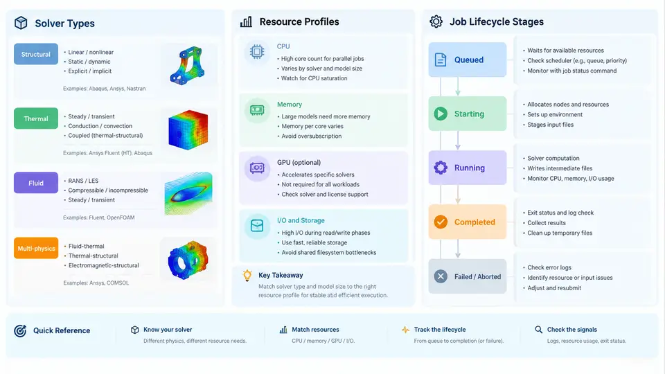
Before any scheduler configuration, submission wrapper, or monitoring dashboard makes sense, you need a precise mental model of what a CAE job actually is on a Linux cluster. A CFD run, an implicit structural solve, and an explicit crash simulation behave very differently in terms of memory access patterns, MPI communication frequency, and I/O burstiness. Treating them as interchangeable "jobs" leads to poor queue design, misleading resource requests, and monitoring rules that fire on the wrong signals. This chapter establishes the vocabulary and the lifecycle model that every later automation decision depends on.
Solver Types and Their Computational Signatures
CAE solvers fall into a small number of families, each with a distinct resource signature. The three most common on Linux HPC clusters are:
- Implicit structural solvers (e.g., Abaqus/Standard, ANSYS Mechanical, Nastran). These assemble and factorize a large sparse stiffness matrix. The dominant cost is the sparse direct solve, which is memory-bandwidth bound and scales poorly beyond a few hundred cores for a single model. Memory per core is high and roughly constant during the solve phase.
- Explicit dynamics solvers (e.g., Abaqus/Explicit, LS-DYNA, Radioss). These advance many small time steps with no global matrix factorization. They are compute-bound, scale well to thousands of cores, and have modest, stable memory footprints. MPI communication is frequent but small.
- CFD solvers (e.g., Fluent, STAR-CCM+, OpenFOAM). These iterate on a mesh-partitioned domain. They are memory-bandwidth bound, sensitive to partition quality, and often produce large transient output files at regular intervals, creating periodic I/O bursts.
A useful way to reason about these differences is to plot them along two axes: parallel scalability and memory intensity. The diagram below places the major solver families in that space and annotates the resource profile each one implies.
The practical consequence is that a single "one size fits all" queue policy is wrong. An implicit structural job requesting 512 cores will waste most of them; an explicit job pinned to 32 cores will run for days when it could finish in hours. Resource requests must be derived from the solver family, not from habit.
Resource Profiles: What to Measure and What to Request
Every job submission carries a resource request. On Slurm this is expressed through directives such as --nodes, --ntasks-per-node, --mem, --time, and --gres. The values you put there should come from a measured profile, not from guesswork. A minimal profile for a solver run includes:
| Dimension | How to measure | Typical implicit | Typical explicit | Typical CFD |
|---|---|---|---|---|
| Peak RSS per rank | /usr/bin/time -v or sacct --format=MaxRSS | 2–8 GB | 0.5–2 GB | 1–4 GB |
| Scaling ceiling | Strong-scaling sweep at 32/64/128/256 cores | ~128–256 | ~1000+ | ~512–2048 |
| Walltime variance | Run 3–5 representative cases | low | low | moderate (convergence) |
| I/O pattern | iostat -x 5 during run | bursty at write | steady, small | periodic large writes |
| Licence tokens | Vendor licence server query | 1 per job | 1 per job | 1 per job + HPC packs |
Two of these deserve emphasis. First, peak RSS is not the same as the memory you should request. Sparse direct solvers can spike during factorization, so request 1.3–1.5× the observed peak. Second, scaling ceiling is the point beyond which adding cores increases walltime. Submitting an implicit job at 512 cores when its ceiling is 200 does not just waste resources — it can make the job slower than a 128-core run because of communication overhead in the factorization.
The Job Lifecycle on a Linux Cluster
A CAE job is not a single event. It passes through a sequence of states, and each state has a different monitoring concern. Understanding this sequence is what makes automation possible — you cannot write a meaningful monitoring rule until you know which state you are watching.
- Preparation. Input deck, mesh, and solver-specific files are staged on shared storage. Pre-processing (partitioning, mesh conversion) may run as a separate short job. Monitoring concern: file integrity and staging latency.
- Submission.
sbatch(orqsub) places the job in the pending queue. The scheduler evaluates priority, fair-share, and resource availability. Monitoring concern: pending reason (sacct -j <jobid> --format=Reason). - Dispatch and launch. The scheduler allocates nodes and launches
mpirun/srun. The solver reads input and begins initialization. Monitoring concern: launch failures, missing libraries, licence checkout errors. - Solve / iterate. The bulk of walltime. The solver writes progress to stdout or a log file. Monitoring concern: convergence rate, residual trends, step time stability.
- Output and post-processing. Results are written to disk; optional post-processing jobs extract fields or generate reports. Monitoring concern: output file size, write errors, disk quota.
- Completion or failure. The job exits with a status code. Monitoring concern: exit code interpretation, partial results, automatic retry decisions.
The critical insight for automation is that states 3 through 5 are where most silent failures occur. A job can be "running" in the scheduler while the solver has actually stalled on a licence checkout, diverged, or filled a disk. Scheduler-level monitoring alone will not catch these; you need solver-level log parsing. This is the core reason the rest of this course builds both layers.
A Worked Example: Profiling a Small Implicit Job
Consider a 2-million-DOF structural model solved with a sparse direct solver. You run it once at 64 cores and once at 128 cores on the same node type, capturing resource usage:
# Run at 64 cores
/usr/bin/time -v srun -n 64 abaqus job=model64 cpus=64 interactive

# Extract key metrics from the Slurm accounting database
sacct -j <jobid> --format=JobID,Elapsed,MaxRSS,MaxVMSize,State,ExitCode
Suppose the 64-core run reports Elapsed=01:12:40, MaxRSS=4.1G per rank, and the 128-core run reports Elapsed=00:58:10, MaxRSS=2.3G per rank. The speedup is only 1.25× for double the cores — well below the 1.4× threshold. The scaling ceiling is therefore near 64 cores for this model. The correct resource request is --ntasks=64 --mem=6G (1.5× the 4.1 GB peak), not 128 cores. This single measurement prevents a systematic over-allocation that would otherwise persist across every similar job.
MaxVMSize. Virtual memory size includes mapped but untouched pages and can be several times larger than actual resident usage. Always use MaxRSS as the basis for --mem.
What This Means for Automation
Three design principles follow directly from the material above. First, resource requests must be solver-aware: a submission wrapper should know whether it is launching an implicit, explicit, or CFD solver and set defaults accordingly. Second, monitoring must operate at two layers: the scheduler layer (is the job running?) and the solver layer (is the solve progressing?). Third, the lifecycle state determines the monitoring action: a pending job needs a different check than a running job, and a completed job needs exit-code interpretation rather than progress parsing.
These principles are the foundation for everything that follows — queue design, submission wrappers, log parsers, and dashboards. The next chapters build each layer in turn, but they all rest on the solver taxonomy and lifecycle model established here.