3. Thermochemical modeling of propellant co
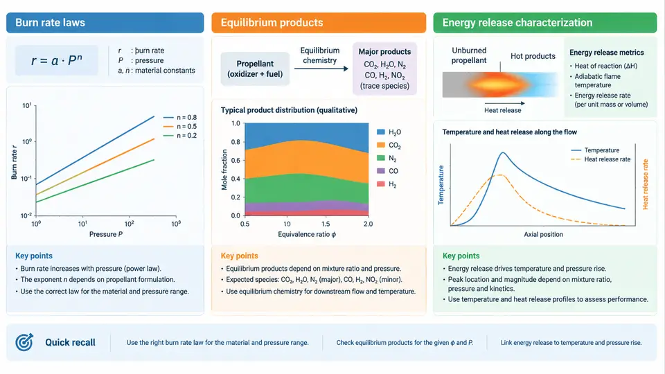
An airbag inflator is, at its core, a small chemical reactor that must discharge its energy within tens of milliseconds. The gas that fills the cushion is not stored gas; it is manufactured on demand by burning a solid propellant. To predict how fast the bag inflates, how hot the gas becomes, and how much toxic by-product leaves the module, the simulation engineer must model three coupled physical processes: the rate at which the solid surface regresses, the equilibrium composition of the resulting gas, and the amount of energy that the reaction releases into that gas. This chapter develops each of these three pillars and shows how they are assembled into a usable inflator model.
Burn Rate Laws: How Fast the Surface Regresses
Solid propellant does not burn in the bulk; it burns only at the exposed surface, and the surface regresses inward at a speed called the linear burn rate r, typically expressed in mm/s. The mass generation rate is then obtained by multiplying the burn rate by the burning surface area Ab and the propellant density ρp:
ṁ_gen = ρ_p · A_b · rThe burn rate itself is a strong function of pressure. The classical empirical description is Saint-Robert's law, also called the Vieille or simply the power law:
r = a · P^nwhere P is the combustion chamber pressure, a is the burn rate coefficient (a temperature-dependent constant), and n is the pressure exponent. For typical sodium azide and non-azide gas generants, n lies between 0.2 and 0.7. The exponent is the single most important stability parameter in the entire model: if n < 1, the system is self-limiting, because a pressure rise increases the burn rate sub-linearly and the chamber tends to settle at an equilibrium pressure. If n ≥ 1, the feedback becomes positive and the inflator can run away. This is why propellant formulators deliberately keep n below unity.
In practice, the simple power law is insufficient over the wide pressure range an inflator experiences, from atmospheric at ignition to 20–40 MPa at peak. Engineers therefore use piecewise fits or the more general Summerfield relation, which introduces a pressure-independent burning rate term. A common practical form used in inflator codes is:
r = a · P^n + bwhere b captures the low-pressure behavior near ignition. The coefficients a, b, and n are obtained from strand-burner tests, in which a small propellant sample is burned in a pressurized vessel and the regression rate is measured optically or by pressure trace. For simulation purposes, these coefficients are the primary calibration inputs, and they must be referenced to a specific initial propellant temperature, since a shifts with temperature according to an Arrhenius-like sensitivity.
Equilibrium Products: What the Propellant Actually Makes
Once the burn rate tells us how much mass is being consumed, we must determine what that mass becomes. Gas generant formulations are complex mixtures—typically a fuel such as guanidine nitrate or sodium azide, an oxidizer such as strontium nitrate or ammonium nitrate, and various additives. The combustion products are not simply the stoichiometric products of a single reaction; they are the composition that minimizes the Gibbs free energy of the mixture at the local temperature and pressure.
The standard approach is equilibrium chemistry, solved by a Gibbs free energy minimizer such as the NASA CEA (Chemical Equilibrium with Applications) code or a real-time reduced-order solver embedded in the inflator model. The solver takes the elemental composition of the propellant (moles of C, H, O, N, and metals per 100 g) and returns the mole fractions of all significant species: CO2, CO, H2O, H2, N2, and trace species such as NOx, NH3, and HCN.
Two features of this equilibrium are critical for airbag modeling. First, the product composition is temperature-dependent, and the temperature is itself a function of the energy release, so the chemistry and the energy balance must be solved simultaneously. Second, the presence of condensed phases—solid or liquid metal oxides such as Na2O, K2O, or SrO—removes material from the gas phase and changes the effective gas yield. A propellant that produces 3.5 mol of gas per 100 g at 2000 K may produce only 3.0 mol per 100 g at 2500 K because more of the oxygen is tied up in condensed oxides.
The practical output of the equilibrium calculation is a table of species mole fractions and a gas yield in moles per unit mass, along with the adiabatic flame temperature Tf. These two quantities are the bridge to the energy release characterization.
Energy Release Characterization
The energy released by combustion is what raises the gas temperature and, through the equation of state, the pressure. The most convenient characterization is the adiabatic flame temperature, defined as the temperature the products would reach if all the chemical energy were released with no heat loss to the surroundings. It is computed from the energy balance:
H_reactants(T_initial) = H_products(T_f)where the enthalpies include the heats of formation of all species. For a typical non-azide gas generant, Tf falls in the range 1800–2600 K. This is the temperature that drives the pressure rise, but it is not the temperature the driver ever sees, because the gas expands, does work on the cushion, and loses heat to the inflator hardware and the filter pack.
For simulation, the energy release is more usefully expressed as the specific energy or impetus of the propellant, often written as F or RTf:
F = n · R · T_fwhere n is the number of moles of gas produced per unit mass and R is the specific gas constant of the mixture. The impetus combines the gas yield and the flame temperature into a single number that directly controls the pressure–time curve. A propellant with a high Tf but a low gas yield may have a lower impetus than a cooler propellant that produces more moles of gas. This trade-off is the central design tension in gas generant formulation.
In a transient inflator model, the energy equation for the combustion chamber is typically written as:
d(m·u)/dt = ṁ_gen · h_p − ṁ_out · h_c − Q_losswhere m is the gas mass in the chamber, u is the specific internal energy, hp is the enthalpy of the generated gas at the flame temperature, hc is the enthalpy of the gas leaving the chamber, and Qloss accounts for heat transfer to the walls and the filter. The equilibrium solver supplies hp and the composition; the burn rate law supplies ṁgen; and the orifice or nozzle model supplies ṁout. The three pillars are thus coupled through the chamber pressure and temperature.
Putting the Three Pillars Together
The following diagram shows how the burn rate law, the equilibrium chemistry, and the energy release characterization interact within a single inflator time step. The burn rate law sets the mass generation; the equilibrium solver determines the composition and flame temperature of that mass; the energy balance converts the chemical energy into a pressure rise; and the pressure feeds back to the burn rate law, closing the loop.
Calibration Workflow and a Worked Example
To make these concepts concrete, consider a hypothetical 60 g non-azide gas generant charge with the following assumed properties: ρp = 1.65 g/cm³, a = 0.045 mm/(s·MPan), n = 0.45, b = 0.8 mm/s, and a burning surface area that starts at 1200 mm² and regresses as the propellant is consumed. The equilibrium solver, given the elemental composition, returns an assumed gas yield of 3.2 mol/100 g and an adiabatic flame temperature of 2250 K at 15 MPa.
The calibration procedure is as follows. First, run the model with the nominal coefficients and compare the predicted pressure–time curve against a closed-vessel (tank) test. Second, if the peak pressure is too low, increase a or the gas yield; if the rise time is too slow, increase n or the burning area. Third, iterate until the predicted and measured curves match within 5 % in peak pressure and 10 % in rise time. The table below summarizes the expected sensitivity of key outputs to each input parameter, based on typical inflator behavior.
| Input Parameter | Typical Range | Effect on Peak Pressure | Effect on Rise Time |
|---|---|---|---|
| Burn rate coefficient a | 0.03–0.08 mm/(s·MPan) | Strong increase | Shorter |
| Pressure exponent n | 0.2–0.7 | Moderate increase | Shorter |
| Gas yield ngas | 2.5–4.0 mol/100 g | Strong increase | Shorter |
| Flame temperature Tf | 1800–2600 K | Moderate increase | Slightly shorter |
| Burning area Ab | 800–2000 mm² | Strong increase | Shorter |
A common failure mode during calibration is a pressure trace that rises too slowly and then overshoots. This usually indicates that the burn rate law is being evaluated at the wrong pressure—often because the model uses the downstream tank pressure instead of the chamber pressure. The chamber pressure is the correct independent variable for r, and it must be computed from the chamber mass balance, not read from the tank. Another frequent issue is a negative or zero gas yield at high temperature, which signals that the equilibrium solver has driven all the oxygen into condensed oxides; in that case, the formulation's oxidizer balance must be revisited.
Key takeaways for the simulation engineer:
- The burn rate law r = a·Pn + b is the primary rate input; n < 1 is required for stable operation.
- Equilibrium chemistry supplies the gas yield and flame temperature, both of which are pressure- and temperature-dependent.
- The energy release is best characterized by the impetus F = n·R·Tf, which couples gas yield and temperature into a single pressure-driving parameter.
- All three pillars are coupled through the chamber pressure and must be solved simultaneously in a transient model.
- Calibration against closed-vessel pressure traces is the standard validation step; peak pressure and rise time are the primary matching criteria.
With the thermochemical model established, the next step in the simulation workflow is to couple it to the gas dynamics of the inflator chamber and the cushion. The burn rate law provides the mass source, the equilibrium solver provides the composition and energy, and the energy balance provides the pressure that drives the flow. Together, these three elements form the predictive core of any airbag inflator model.