3. PAM-CRASH material model selection for f
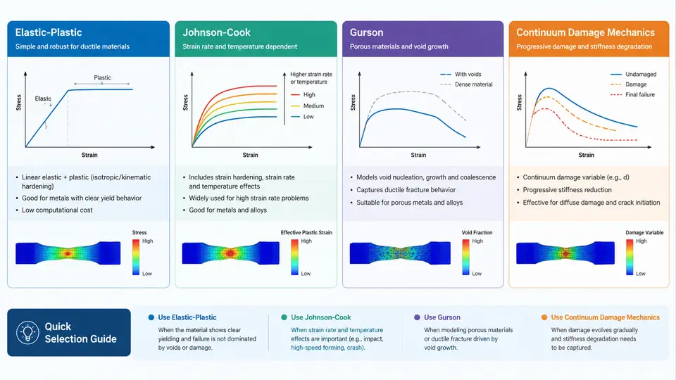
Selecting a constitutive model in PAM-CRASH is not a matter of picking the most sophisticated option available. It is a decision about which physical mechanisms dominate the failure event you are trying to predict, and which of those mechanisms the available material data can actually calibrate. A model that captures void growth beautifully is useless if you only have tensile test data at a single strain rate. This section walks through the four families most commonly used for failure and damage work in PAM-CRASH — elastic-plastic, Johnson-Cook, Gurson-type porous plasticity, and continuum damage mechanics (CDM) — and gives you a practical basis for choosing among them.
Elastic-Plastic Models: The Baseline
The elastic-plastic family (material types such as 101, 102, and their variants) treats failure through a simple criterion: a scalar equivalent plastic strain threshold, optionally with a stress-state or element-size correction. The yield surface is typically von Mises, hardening is tabulated as stress versus plastic strain, and failure occurs when the accumulated plastic strain at an integration point exceeds a user-defined value.
This is the right choice when the material is ductile, the stress triaxiality stays within a moderate band, and you mainly need to know where and roughly when rupture initiates. It is also the only defensible choice when your calibration data is limited to a uniaxial tensile curve. The limitation is equally clear: a single plastic strain limit cannot distinguish between a shear-dominated and a tension-dominated loading path, so predictions degrade badly in crash scenarios with mixed-mode loading.
A typical setup uses a piecewise-linear hardening table and a failure strain that is adjusted for element size. If your shell mesh has a characteristic length of 2 mm and the tensile coupon's gauge length was 50 mm, the failure strain must be scaled — otherwise the mesh will localize and the result becomes mesh-dependent. PAM-CRASH provides regularization options, but they only work if you supply a consistent characteristic length.
Johnson-Cook: Strain Rate and Temperature
Johnson-Cook (JC) extends the elastic-plastic framework with explicit strain-rate and temperature dependence. The flow stress is written as a product of three terms: a strain-hardening term, a rate-sensitivity term, and a thermal-softening term. Failure is handled by a separate JC damage criterion in which the equivalent plastic strain at fracture depends on stress triaxiality, strain rate, and temperature.
Choose JC when the loading is dynamic — automotive crash, impact, blast — and when you have data at more than one strain rate. The rate term is usually calibrated from split Hopkinson pressure bar tests or high-rate tensile tests, and the thermal term from elevated-temperature tests. If you only have quasi-static data, the rate term collapses to unity and JC degenerates into a rate-independent model with a more flexible failure surface than the simple elastic-plastic option.
The practical pitfall is over-parameterization. JC has five flow-stress constants and five damage constants. Fitting all ten from a single test series produces a model that interpolates the calibration data well and extrapolates poorly. A defensible workflow fixes the elastic constants from standard tests, fits the hardening term from quasi-static data, then fits the rate term from dynamic data, and only then fits the damage constants. Each stage should be validated against a test not used in the fit.
Gurson and Porous Plasticity: Ductile Fracture by Void Growth
Gurson-type models (including the GTN extension with nucleation, growth, and coalescence parameters) describe ductile fracture as the evolution of a void volume fraction. The yield surface is pressure-sensitive: hydrostatic tension accelerates void growth, while hydrostatic compression suppresses it. Failure occurs when the void volume fraction reaches a critical value, at which point the material loses load-carrying capacity.
This is the model to use when the failure mode is genuinely void-dominated — cup-and-cone tensile fracture, ductile tearing in sheet metal, or damage accumulation under high triaxiality. It is also the model of choice when you need to predict the softening phase before final fracture, not just the onset. The cost is calibration burden: you need the initial void fraction, the critical and final void fractions, and nucleation parameters, typically obtained from metallography, density measurements, or inverse fitting against notched tensile tests.
Gurson models are computationally heavier and more sensitive to mesh size than JC. They are rarely the right first choice for a full-vehicle crash model, but they are excellent for component-level studies where the fracture mechanism matters.
Continuum Damage Mechanics: Stiffness Degradation
CDM models represent damage as a scalar or tensorial internal variable that degrades stiffness. Instead of a sudden failure criterion, the material progressively loses stiffness as damage accumulates, and the stress-strain response softens. In PAM-CRASH, CDM options are often used for composites, adhesive joints, and materials where distributed micro-cracking precedes final rupture.
The strength of CDM is that it captures the gradual loss of load path, which matters for structures that redistribute load after local damage. The weakness is that damage evolution laws introduce regularization problems: without a characteristic length or viscous regularization, the damage zone localizes to a single element row and the result becomes mesh-dependent. If you use CDM, you must address regularization explicitly.
Choosing Among the Four
The decision can be organized around three questions: what is the dominant failure mechanism, what data do you have, and what output do you need?
| Model family | Dominant mechanism | Minimum data | Best for | Main risk |
|---|---|---|---|---|
| Elastic-plastic | Ductile rupture, moderate triaxiality | Tensile curve, failure strain | Baseline crash models, screening | Mesh-dependent failure strain |
| Johnson-Cook | Rate- and temperature-dependent ductile fracture | Multi-rate tests, temperature tests | Impact, blast, high-rate crash | Over-fitting ten constants |
| Gurson / GTN | Void growth and coalescence | Void fraction, notched tests | Component-level ductile tearing | Calibration cost, mesh sensitivity |
| CDM | Progressive stiffness degradation | Damage evolution data | Composites, adhesives, distributed damage | Localization without regularization |
A useful discipline is to start with the simplest model that can represent the mechanism, run a validation case against a test not used in calibration, and only escalate to a more complex model if the simple one fails in a way that the complex model's extra physics would fix. Escalating because the simple model is "not accurate enough" without identifying which mechanism is missing usually produces a more expensive model with the same error.
Calibration and Validation Workflow
Regardless of which model you choose, the workflow has the same shape. First, fix the elastic constants from standard tensile or ultrasonic data — these should not be tuned during failure calibration. Second, calibrate the plasticity or damage evolution using the test that most directly probes the mechanism. Third, calibrate the failure criterion using a test with a different stress state, such as a notched or shear specimen. Fourth, validate against a third test that was not used in any fit.
For a JC model applied to a typical automotive steel, a defensible starting point might be: E = 210 GPa, ν = 0.3, A = 350 MPa, B = 600 MPa, n = 0.5, C = 0.015, m = 1.0, with damage constants D1 through D5 fitted from notched tensile tests at two rates. These values are illustrative and must be replaced with actual calibration data for any real project. The point is the structure of the parameter set, not the numbers.
When results look wrong, the diagnostic order matters. If the failure location is wrong, suspect the stress-state dependence of the criterion. If the failure timing is wrong but the location is right, suspect the hardening or rate term. If the result changes significantly when you refine the mesh, suspect missing regularization. If the model runs but produces no failure at all, check that the failure criterion is actually activated and that the element deletion flag is set.
The four families are not a ladder of increasing quality. They are different physical hypotheses. Elastic-plastic assumes failure is governed by accumulated plastic strain alone. Johnson-Cook adds rate and temperature. Gurson adds void mechanics. CDM adds progressive stiffness loss. The correct choice is the one whose hypothesis matches your failure mechanism and whose parameters your data can support.