1. Full vehicle frontal impact simulation i
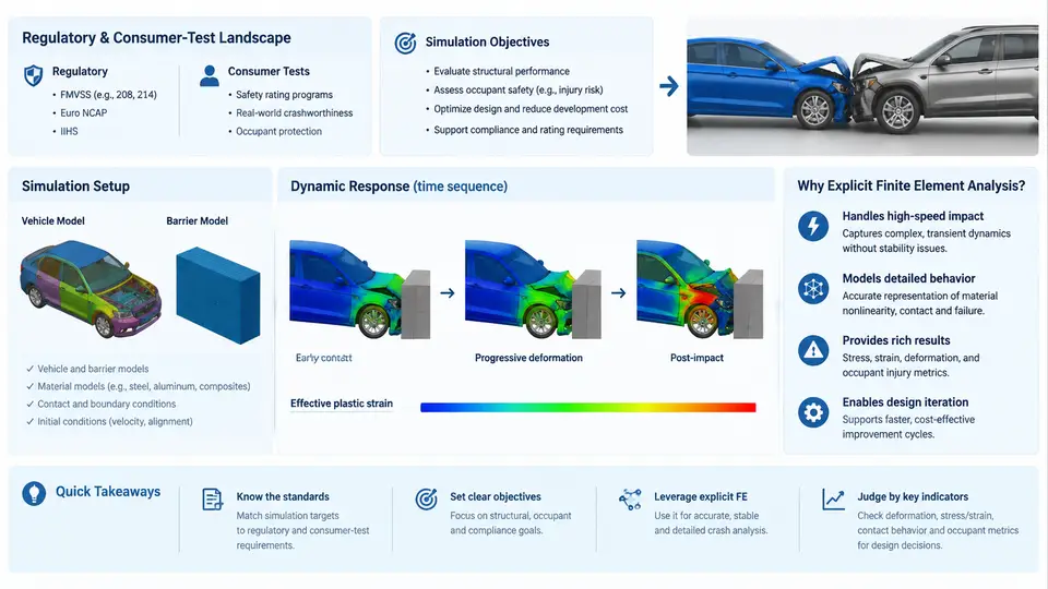
Full vehicle frontal impact simulation sits at the intersection of crashworthiness regulation, consumer rating programs, and high-performance explicit finite element (FE) computation. Before a single element is meshed, an engineer must understand why the simulation exists: which load case is being reproduced, which injury or structural metric must be predicted, and which numerical method can deliver that prediction within an acceptable turnaround time. This chapter establishes that foundation and frames the rest of the course.
The Regulatory and Consumer-Test Landscape
Frontal impact requirements come from two distinct but overlapping sources. Homologation regulations define the legal minimum a vehicle must satisfy to be sold. In Europe, UNECE Regulation No. 94 specifies a 40% offset deformable barrier (ODB) test at 56 km/h; in the United States, FMVSS 208 covers full frontal rigid barrier impacts at 56 km/h (35 mph) plus offset and angled variants, with occupant restraint performance assessed through instrumented Anthropomorphic Test Devices (ATDs, or "dummies"). Consumer-test programs — Euro NCAP, US NCAP, C-NCAP, and IIHS — go further, using higher severities, additional configurations, and star ratings that directly influence market perception.
Two configurations dominate frontal work:
- Full frontal rigid barrier (FRB): the entire vehicle front contacts a fixed, non-deformable wall. Load is distributed across the full width; the primary concern is occupant deceleration and restraint system performance.
- Offset deformable barrier (ODB): only part of the front structure engages a crushable barrier, producing asymmetric loading, longitudinal rail bending, and a higher risk of structural intrusion into the occupant compartment.
Euro NCAP's frontal ODB test runs at 64 km/h with a 40% overlap against a honeycomb barrier, while the mobile progressive deformable barrier (MPDB) test introduced in recent protocols adds a moving trolley to evaluate compatibility between vehicles of different masses. IIHS uses a 25% small overlap rigid barrier at 64 km/h, which bypasses the main longitudinal rails and loads the wheel, suspension, and firewall directly — a case that historically exposed weaknesses in many designs.
Simulation Objectives
A frontal impact simulation is not a single analysis but a set of coupled predictions. The objectives typically include:
- Structural integrity: predict crush mode, longitudinal rail folding, and whether the occupant compartment (footwell, A-pillar, dash panel) intrudes beyond a defined limit.
- Occupant kinematics and injury criteria: derive dummy responses — Head Injury Criterion (HIC), chest deflection, femur loads, neck injury (Nij) — from the simulated motion.
- Restraint system performance: verify airbag deployment timing, seatbelt load limiting, and pretensioner behavior interact correctly with the deforming structure.
- Energy management: confirm that kinetic energy is absorbed through controlled plastic deformation rather than transferred to occupants or causing component separation.
- Design comparison: evaluate material grades, gauge thickness, and geometry changes before committing to physical prototypes.
These objectives drive the model's required fidelity. A rail crush study may tolerate a coarser mesh, but an injury-criteria prediction demands accurate dummy positioning, contact definitions, and material strain-rate data.
Why Explicit Finite Element Analysis
Frontal impact is a transient, highly nonlinear event lasting roughly 80–150 ms. It involves large plastic deformation, self-contact, strain-rate-sensitive materials, and geometric nonlinearity. The implicit solvers used for static stiffness analysis cannot handle this efficiently because each Newton-Raphson iteration requires solving a large system of equations, and convergence becomes fragile once elements distort severely.
Explicit FE analysis, the method PAM-CRASH implements, reformulates the equations of motion so that the acceleration of each node is computed directly from the internal and external forces acting on it:
M · a = F_ext − F_int
a = M⁻¹ · (F_ext − F_int)
Because the mass matrix M is lumped (diagonal), its inverse is trivial, and no global matrix factorization is needed. The solution advances with a central-difference time integration scheme, and stability requires the time step to satisfy the Courant–Friedrichs–Lewy (CFL) condition:
Δt ≤ L_min / c
c = √(E / ρ)
where L_min is the smallest element characteristic length, c is the speed of sound in the material, E is Young's modulus, and ρ is density. A typical steel model with a 5 mm element yields a stable time step on the order of 1 µs, meaning a 100 ms event requires roughly 100,000 increments. This is why explicit crash simulation is computationally intensive and why mass scaling, subcycling, and selective mesh refinement are standard practice.
The explicit approach also handles contact naturally: penalty-based or kinematic contact algorithms detect penetrations at each increment and apply restoring forces, which suits the many self-contacting surfaces in a crushed vehicle. PAM-CRASH's architecture — with its material library covering elastoplasticity, strain-rate dependence, failure, and spot-weld/ adhesive rupture — is built specifically for this class of problem.
From Test Protocol to Simulation Model
Translating a test protocol into a PAM-CRASH model requires several deliberate decisions. The barrier must be represented with the correct geometry and material: a rigid wall for FRB, or a honeycomb block with calibrated crush stress for ODB. The initial velocity is applied to the entire vehicle as a prescribed initial condition, and gravity is included to capture the pre-impact attitude. The dummy is positioned per the protocol's seating procedure, and its FE model must match the certification dummy's mass distribution and joint stiffness.
Boundary conditions matter: the ground plane is modeled as a rigid surface with friction, and the vehicle's suspension is either represented explicitly or simplified with kinematic constraints depending on whether suspension failure is part of the study. Output requests are defined before the run — nodal displacements at the firewall, section forces in the rails, accelerometer signals at the B-pillar and seat tracks, and dummy injury channels.
What the Simulation Must Deliver
By the end of a frontal impact study, the engineer should be able to answer concrete questions: Does the firewall intrude past the 150 mm limit? Does the airbag fire early enough to catch the head before it reaches the steering wheel? Is the rail folding in a stable, progressive mode, or is it bending globally and losing energy-absorption capacity? These answers come from post-processing the d3plot-equivalent result files, extracting time histories, and comparing them against physical test data or program targets.
The remainder of this course builds on this foundation: model setup, material calibration, contact definition, dummy positioning, and result validation. Each subsequent chapter assumes the reader understands that the simulation is not an end in itself — it is a predictive tool whose credibility depends on how faithfully the test landscape, the objectives, and the explicit solver's numerical constraints are respected.