3. Material modeling for crashworthiness
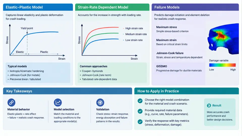
Crashworthiness simulation is only as trustworthy as the constitutive response assigned to each material. In a frontal impact model, the difference between a structure that folds progressively and one that fractures prematurely usually comes down to three modeling decisions: how the material hardens after yield, how strongly it responds to strain rate, and when it is allowed to fail. PAM-CRASH provides dedicated material laws for each of these behaviors, and this section explains what those laws represent, how their parameters are obtained, and how to select and calibrate them for a typical body-in-white application.
The Three Pillars of a Crash Material Law
Every crashworthiness material model in PAM-CRASH can be decomposed into three functional blocks that act in sequence as strain increases. The elastic-plastic block defines the yield surface and the hardening curve, converting total strain into an equivalent plastic strain and a flow stress. The strain-rate block scales that flow stress according to the current deformation velocity, which is essential because mild steel at 10 s⁻¹ can be 30–50 % stronger than in a quasi-static tensile test. The failure block decides when the element loses load-carrying capacity, either by deleting it or by degrading its stiffness. These blocks are not independent in practice: a rate-dependent model with no failure criterion will absorb far more energy than the real component, while an aggressive failure criterion on a rate-insensitive model will trigger too early in high-speed events.
Elastic-Plastic Models: MAT 103 and MAT 105
The workhorse for ductile metals in PAM-CRASH is MAT 103 (elastic-plastic isotropic), often used with shell elements for stamped steel and aluminium panels. It requires the elastic modulus E, Poisson's ratio ν, initial yield stress σ_y, and either a constant tangent modulus E_t or a piecewise hardening curve given as true stress versus true plastic strain. For crash analysis, the piecewise form is strongly preferred because the difference between a bilinear approximation and the real curve can shift absorbed energy by 10–15 % in a folding rail.
To build the hardening input, convert the engineering stress–strain curve from the tensile test into true stress and true plastic strain using σ_true = σ_eng(1+ε_eng) and ε_pl = ln(1+ε_eng) − σ_true/E. The curve should be extrapolated beyond necking up to the failure strain expected in the component, typically 0.3–0.6 for deep-drawn mild steel. MAT 105 (elastic-plastic kinematic) adds a kinematic hardening term and is the better choice when the structure experiences load reversal or cyclic bending, such as a rocker panel in a side impact. A common pitfall is using MAT 103 with a hardening curve that was truncated at uniform elongation; the model then behaves almost perfectly plastic in the post-necking regime and over-predicts energy absorption.
Strain-Rate Dependent Models: Cowper-Symonds and Tabulated Curves
Rate sensitivity is introduced in PAM-CRASH through the Cowper-Symonds relation, which scales the flow stress by a factor R = 1 + (ε̇/D)^(1/q). For typical automotive mild steel, D ≈ 40 s⁻¹ and q ≈ 5; for high-strength steel, D rises to several hundred and q to 6–8, meaning the material is less rate-sensitive. These constants are fitted from Split Hopkinson Pressure Bar (SHPB) tests at strain rates of 100–5000 s⁻¹, supplemented by intermediate-rate servo-hydraulic tests at 1–100 s⁻¹.
When a single Cowper-Symonds pair cannot capture the full rate range, PAM-CRASH allows a tabulated rate-scaling curve, where the amplification factor is read directly from a table of ε̇ versus R. This is the more accurate route for aluminium alloys, whose rate sensitivity saturates above roughly 1000 s⁻¹. A practical check after calibration is to run a single-element simulation at three rates (0.001, 1, 1000 s⁻¹) and confirm that the predicted flow stress matches the test data within 5 %.
Failure Models: From Simple Plastic Strain to GISSMO
The simplest failure option is a plastic strain at failure criterion, where the element is deleted once equivalent plastic strain reaches a fixed value. This is adequate for preliminary studies but ignores stress triaxiality, so it fails to distinguish between a shear-dominated and a tension-dominated fracture path. For crashworthiness work, the recommended model is GISSMO (Generalized Incremental Stress State dependent damage model), available in PAM-CRASH as MAT 124 or through the GISSMO add-on. GISSMO accumulates damage D = Σ Δεᵖ / ε_f(η, ε̇), where the failure strain ε_f depends on stress triaxiality η = σ_m / σ_vm and strain rate. The failure locus is calibrated from a set of specimen geometries: smooth tensile (η ≈ 0.33), notched tensile (η ≈ 0.5–0.7), shear (η ≈ 0), and biaxial (η ≈ 0.67).
GISSMO also supports a damage-induced softening phase, where stiffness is degraded before final rupture. This is important for predicting the post-initiation response of a component that has already cracked but still carries load. The instability strain ε_inst controls when softening begins, and the softening exponent m controls how quickly the stress drops. Typical values for dual-phase steel are ε_inst ≈ 0.15–0.25 and m ≈ 2–4.
Selecting and Calibrating a Material Card: A Worked Example
Consider a front longitudinal rail made of DP600, 1.8 mm thick, modeled with 5 mm shell elements. The calibration workflow is:
- Hardening: Fit the true stress–plastic strain curve from a quasi-static tensile test up to
ε_pl = 0.5. Use MAT 103 with the piecewise curve. - Rate: Fit Cowper-Symonds constants from SHPB data. For DP600, a reasonable starting point is
D = 800 s⁻¹,q = 6.5. Verify with single-element runs at 1 and 1000 s⁻¹. - Failure: Calibrate the GISSMO failure locus from notched and shear specimens. Set
ε_inst = 0.20,m = 3. - Validation: Run a drop-tower simulation of the rail at 15 m/s and compare the force–displacement curve and the final fold pattern against the physical test. A good match shows a peak force within 8 % and the same number of folds.
Practical Checks Before Running the Full Model
Before committing to a full vehicle run, perform three quick checks. First, run a single-element tension test in PAM-CRASH and overlay the predicted stress–strain curve on the experimental data; the curves should coincide up to the failure strain. Second, run a three-point bending simulation of a small coupon and verify that the force–displacement response matches the test within 10 %. Third, inspect the material card for unit consistency: PAM-CRASH uses consistent units, so if the geometry is in millimeters and the density in kg/mm³, the stress must be in MPa and the strain rate in s⁻¹. A unit mismatch is the most common cause of a model that runs but produces nonsensical energy absorption.
With the material card calibrated and validated at the coupon level, the model is ready for component and full-vehicle crash simulation. The next step is to assemble these material definitions into a complete crash model and verify that the global energy balance remains physical throughout the event.