1. Build a Baseline Sled Model and Correlat
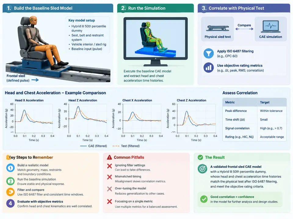
Baseline Sled Model Scope and Correlation Target
This first case establishes the reference model that every later correlation exercise will build on. The task is narrow but demanding: assemble a frontal sled CAE model with a Hybrid III 50th percentile male dummy, run one baseline simulation, and compare the simulated head and chest resultant accelerations against a physical sled test using ISO 6487 channel filtering and objective rating metrics. The deliverable is not a "good-looking" animation — it is a defensible statement of how far the baseline model is from test, expressed in numbers that can be tracked as the model is improved in later cases.
Two conventions must be fixed before any work begins, because every downstream comparison depends on them:
- Sign convention: the vehicle forward direction is +X. The dummy faces +X. Head and chest accelerations are reported as resultant magnitudes (always positive) for rating, but the signed X components are retained for time-history plots so that phase and polarity errors are visible.
- Time zero: t = 0 is defined as the first sample at which sled acceleration exceeds 0.5 g. Both test and CAE channels are shifted to this reference before any metric is computed. A 5 ms misalignment at this stage will corrupt every cross-correlation value later.
Model Assembly: What Must Be Present and Correct
A baseline sled model that can be correlated has five subsystems that must each be individually sanity-checked before the run. Skipping any one of them produces a correlation failure that is impossible to attribute.
| Subsystem | Key objects | Baseline check before running |
|---|---|---|
| Sled / buck | Rigid sled platform, seat frame, floor pan, knee bolster, toe pan | Total mass within 2% of test buck mass; prescribed acceleration pulse applied to sled node set |
| Restraint | Retractor, shoulder belt, lap belt, buckle, anchor points | Belt path matches test routing; initial belt slack and pretensioner stroke set to test values |
| Dummy | Hybrid III 50th percentile FE model, positioning joints, contact definitions | H-point and seat back angle match test setup sheet; limb angles within 2° of test photos |
| Contact | Dummy-to-seat, dummy-to-belt, dummy-to-knee bolster | No initial penetration; friction coefficients set from test hardware (belt-to-dummy μ ≈ 0.3, dummy-to-seat μ ≈ 0.5) |
| Output | Head CG accelerometer, chest accelerometer triad, sled accelerometer | Requested at the same sample rate as test (typically 10 kHz), with ISO 6487 CFC 1000 filter applied post-run |
The most common baseline error is a mass mismatch. If the sled plus buck mass differs from the test by more than a few percent, the prescribed pulse will produce a different velocity change (ΔV), and every acceleration comparison will be biased. Compute ΔV by integrating the pulse and compare it to the test-reported ΔV before proceeding.
Running the Baseline and Extracting Comparable Channels
Run the simulation with the prescribed pulse and confirm the run terminates normally with no negative-volume or mass-scaling warnings that would invalidate the result. Then extract three channels: sled X acceleration, head CG resultant acceleration, and chest resultant acceleration. Apply ISO 6487 CFC 1000 filtering to the CAE channels using the same filter implementation and phase correction as the test data reduction. Do not compare unfiltered CAE output to filtered test data — this alone can create apparent 10–15% magnitude errors at peak.
# Example channel extraction and ISO 6487 CFC 1000 filtering (Python, scipy)
import numpy as np
from scipy import signal

def cfc1000_filter(t, a):
    # ISO 6487 CFC 1000: 4th-order Butterworth, fc = 1650 Hz, zero-phase
    fs = 1.0 / (t[1] - t[0])
    fc = 1650.0
    b, a_coef = signal.butter(4, fc / (fs / 2.0), btype='low')
    return signal.filtfilt(b, a_coef, a)

# Load CAE and test channels (columns: time_s, sled_ax, head_res, chest_res)
cae  = np.loadtxt('baseline_cae.csv', delimiter=',', skiprows=1)
test = np.loadtxt('sled_test_01.csv', delimiter=',', skiprows=1)

# Align to t=0 at first sample exceeding 0.5 g on sled channel
def align(t, sled_ax):
    idx = np.argmax(np.abs(sled_ax) > 0.5 * 9.81)
    return t - t[idx]

cae[:, 0]  = align(cae[:, 0],  cae[:, 1])
test[:, 0] = align(test[:, 0], test[:, 1])

head_cae_f  = cfc1000_filter(cae[:, 0],  cae[:, 2])
chest_cae_f = cfc1000_filter(cae[:, 0],  cae[:, 3])
head_tst_f  = cfc1000_filter(test[:, 0], test[:, 2])
chest_tst_f = cfc1000_filter(test[:, 0], test[:, 3])
Resample both filtered sets onto a common 0.1 ms grid over the 0–150 ms window before computing metrics. This removes any dependence on differing native sample rates and makes the correlation metrics reproducible.
Objective Rating: What the Numbers Mean
Two metrics are sufficient for a baseline and are the ones to carry forward. The peak value ratio (CAE peak / test peak) tells you whether the model over- or under-predicts severity. The cross-correlation factor (the maximum of the normalized cross-correlation over a ±15 ms lag window) tells you shape and phase agreement independent of amplitude. Report both, plus the lag at which the maximum occurs — a consistent lag across head and chest usually points to a timing issue in the pulse or belt engagement, not a dummy property error.
Interpreting a Baseline Result and Recording It
Suppose the baseline run returns a head peak ratio of 1.09 with a cross-correlation factor of 0.91 at a lag of +3 ms, and a chest peak ratio of 0.88 with a cross-correlation factor of 0.86 at a lag of +7 ms. The head passes all three gates. The chest passes amplitude and shape but fails the lag gate at +7 ms. The correct interpretation is not "tune the chest" — it is that the chest channel is rising later than test, which most often traces to belt slack, retractor spool-out timing, or a seat back angle that lets the torso rotate before the belt engages. Record this as the baseline finding; the belt system is the subject of the next case, so the lag is expected to be addressed there rather than by ad-hoc dummy tuning.
If instead the head peak ratio came back at 1.35 with a cross-correlation factor of 0.72, the shape is wrong, not just the amplitude. Before touching any parameter, verify the filter was applied to the CAE channel and that the pulse ΔV matches test. An unfiltered CAE head channel routinely over-predicts peak by 20–30% and produces exactly this signature.
Baseline Record Sheet
Capture the following for the baseline so that every later case can be compared against a fixed reference. Fill the values from the actual run; the structure below is the minimum record.
| Field | Head resultant | Chest resultant |
|---|---|---|
| Test peak (g) | — | — |
| CAE peak, CFC 1000 (g) | — | — |
| Peak ratio | — | — |
| Cross-correlation factor | — | — |
| Lag at max correlation (ms) | — | — |
| Gate result (pass/fail) | — | — |
| Observed failure mode | — | — |
Also record the sled pulse ΔV (CAE vs test), the buck mass difference, and the dummy H-point offset. These three numbers explain most baseline failures and are the first things to check when a later case's correlation unexpectedly degrades.
baseline_v1. Every subsequent correlation case should diff against this tag, not against a re-run, so that improvements are attributable to the parameter change under study rather than to incidental model edits.