1. Yield optimization in manufacturing
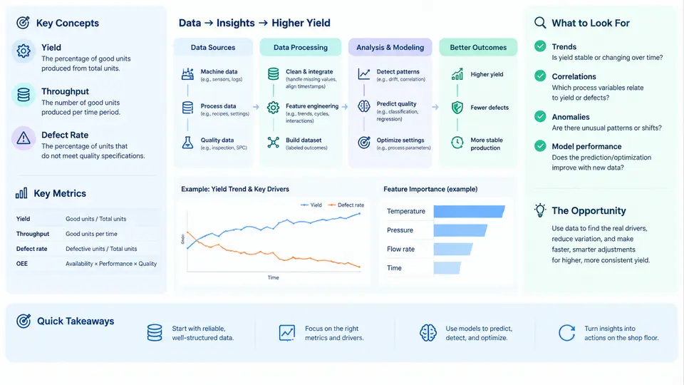
Yield is the single number that most directly connects a factory's process capability to its profitability. In semiconductor, electronics assembly, pharmaceutical, and precision-machining environments, yield answers a deceptively simple question: of everything we started, how much came out good? Yet the way that question is framed — at which step, over which window, with which definition of "good" — determines whether the metric drives real improvement or merely decorates a dashboard. This chapter establishes the vocabulary, the metric hierarchy, and the specific places where data science changes what a yield team can actually do.
What Yield Actually Means
At its core, yield is a ratio of conforming output to total input. The complication is that a modern production line has dozens of steps, and a unit can be lost at any of them. Three definitions dominate practice:
- First-pass yield (FPY) — the fraction of units that pass a given step or the entire line on the first attempt, without rework, retest, or repair. FPY is the honest measure of process health because it refuses to hide defects behind rework loops.
- Rolled throughput yield (RTY) — the product of the individual step yields across a sequence. If five steps each yield 95%, RTY = 0.95⁵ ≈ 77.4%. This multiplicative behavior is why a line of individually "good" steps can still deliver poor final yield, and it is the first place where a data-driven view pays off.
- Final yield — conforming units at the end divided by units started, after rework is counted. Final yield flatters a process; FPY and RTY expose it.
For a worked example, consider a five-step assembly line with step yields of 0.98, 0.96, 0.99, 0.94, and 0.97. RTY = 0.98 × 0.96 × 0.99 × 0.94 × 0.97 ≈ 0.849, or 84.9%. Improving the weakest step (0.94) to 0.97 raises RTY to roughly 0.876 — a 2.7-point gain from a single step. This sensitivity analysis, done across all steps, is the simplest form of yield optimization and requires nothing more than the step-yield table.
The Metric Hierarchy
Yield alone is insufficient because it says nothing about why units fail or how close passing units were to the limit. A practical metric stack pairs yield with defect and capability measures:
| Metric | Definition | What it reveals |
|---|---|---|
| FPY / RTY | First-pass and rolled throughput yield | Process health without rework masking |
| DPPM / DPMO | Defective parts per million / defects per million opportunities | Defect density, comparable across product complexity |
| Cpk / Ppk | Process capability vs. specification limits | How much margin exists before failures appear |
| Defect Pareto | Failure modes ranked by frequency or cost | Where to focus improvement effort |
| Excursion rate | Frequency of out-of-control events per tool or lot | Stability of the process over time |
Cpk deserves emphasis because it is the leading indicator that yield is about to move. Cpk = min[(USL − μ), (μ − LSL)] / (3σ). A process running at Cpk = 1.33 has roughly 63 DPPM if centered; at Cpk = 1.0, that rises to about 2,700 DPPM. Yield is the lagging result; Cpk and defect density are the leading signals. A yield program that only watches yield is always reacting.
Where the Data Science Opportunity Lives
Traditional yield engineering relies on designed experiments, control charts, and engineer intuition. These remain essential, but they scale poorly against the realities of modern fabs and assembly lines: hundreds of process steps, thousands of sensors, trace data at millisecond resolution, and defect signatures that span multiple tools and lots. The data science opportunity is not "replace the engineer" — it is to compress the time between a yield loss occurring and its root cause being identified, and to predict losses before they happen.
Four concrete opportunity areas dominate:
- Yield prediction from process and sensor data. Models trained on inline metrology, tool sensor traces, and historical yield labels can flag lots at risk before final test. A typical setup uses features such as chamber temperature deviation, deposition rate, and queue time between steps, with a gradient-boosted classifier predicting pass/fail at the next inspection point.
- Root-cause and commonality analysis. When yield drops, the question is which tool, chamber, lot, or recipe is shared by the failing units. Automated commonality scoring across tool history and defect maps replaces days of manual slicing.
- Spatial defect pattern recognition. Wafer maps and board images carry signatures — edge rings, center clusters, scratch lines — that correspond to specific mechanisms. Convolutional models classify these patterns and link them to process drift.
- Prescriptive optimization. Once relationships are quantified, setpoint and scheduling decisions can be tuned to maximize RTY subject to constraints, rather than adjusted by trial and error.
The figure below shows how these pieces connect: raw process and test data feed a feature and label layer, which supports both prediction and diagnosis, and the outputs feed back into process control and scheduling decisions that determine the next yield result.
A Minimal Working Example
To make the loop concrete, suppose a team wants to predict final-test failure for a lot using inline data. The reproducible setup is:
Inputs:
  - lot_id, tool_id, chamber_id, recipe_id
  - inline metrology: film_thickness_nm, cd_nm, overlay_nm
  - tool trace summary: temp_mean_c, temp_std_c, pressure_mean_torr
  - queue_time_hours between critical steps
  - label: final_test_pass (0/1)

Steps:
  1. Join metrology and trace summaries to lot_id.
  2. Compute step-level yield and Cpk per tool/chamber over a rolling 30-day window.
  3. Train a gradient-boosted classifier with 5-fold cross-validation.
  4. Evaluate with precision/recall at the operating threshold, not accuracy.
  5. Rank feature importances and cross-check against known mechanisms.

Expected observable output:
  - A ranked list of at-risk lots with a risk score.
  - Feature importances showing which parameters drive failure.
  - A confusion matrix at the chosen threshold.

Typical failure symptoms and checks:
  - High accuracy but near-zero recall: class imbalance; reweight or resample.
  - Importances dominated by lot_id or timestamp: leakage; remove identifiers.
  - Model degrades after deployment: process drift; monitor input distributions.
The point of this example is not the specific algorithm. It is that yield optimization becomes tractable when the problem is framed as a labeled prediction task with a clear evaluation criterion and a defined feedback path into process control. The remaining chapters build out each stage of this loop in depth.
With the definitions, the metric hierarchy, and the data science loop established, the next step is to understand where the data itself comes from and what limits its quality — the subject of the following chapter.