4. Sled pulse generation and control
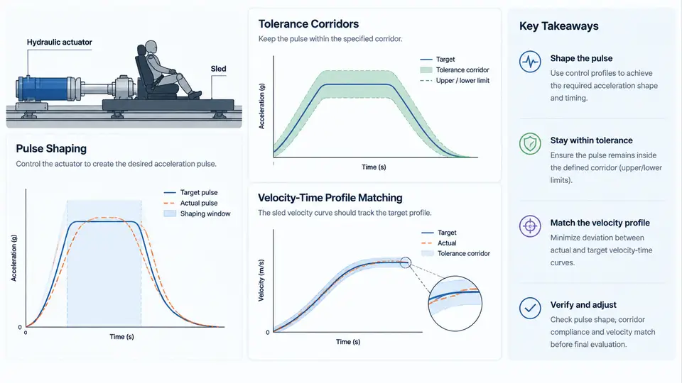
A crash sled test is only as meaningful as the acceleration pulse it reproduces. The sled pulse is the prescribed deceleration (or acceleration) history applied to the test buck, and it defines the inertial loading that every restraint component — belt, airbag, pretensioner, load limiter, seat structure — will experience. If the pulse is wrong, the restraint system is evaluated against the wrong physics, and the resulting pass/fail judgment is invalid. This chapter explains how pulses are generated, how they are shaped to match a target, how tolerance corridors define acceptable deviation, and how the velocity–time profile is verified against the intended crash severity.
4.1 What a Sled Pulse Actually Is
A sled pulse is a time-domain acceleration signal, typically expressed in g (1 g = 9.81 m/s²), applied along the primary longitudinal axis. In a deceleration-type sled, the buck is accelerated to a target velocity and then decelerated by a programmable energy-absorbing device. The recorded signal is the sled table acceleration a(t). Two derived quantities matter as much as the raw acceleration:
- Velocity change ΔV = ∫a(t)dt over the pulse duration. This is the crash severity the occupant actually "sees."
- Displacement s(t) = ∫∫a(t)dt², which must remain within the sled's stroke budget.
The sign convention must be fixed before any analysis. In this course, deceleration is treated as positive magnitude along the vehicle's forward axis, and the sled travels in the +X direction before decelerating. All corridors, integrals, and plots in this chapter follow that convention. If a test house uses the opposite sign, the corridor must be mirrored, not merely relabeled.
4.2 Pulse Shaping Methods
Pulse shape is controlled by the energy absorber between the sled and the reaction structure. Three families dominate:
| Method | Shaping mechanism | Typical use |
|---|---|---|
| Hydraulic servo | Programmable valve controls orifice area vs. stroke | Highly repeatable, complex waveforms |
| Metal tube/plate deformation | Plastic folding or tearing of a sacrificial member | Rugged, low-cost, fixed-ish shape |
| Composite/foam crush | Progressive crushing of a tuned coupon stack | Fast tuning, moderate repeatability |
For a hydraulic system, the engineer specifies a target waveform and the controller solves for the valve command that produces it. For a deformation-based absorber, shaping is done by selecting material, wall thickness, and geometry. A common practical approach is to start from a coupon test: crush a candidate tube at quasi-static and dynamic rates, record its force–displacement curve, then convert force to acceleration using the sled mass.
a(t) = F_absorber(t) / m_sled_total

where:
  F_absorber(t) = measured crush/deformation force [N]
  m_sled_total  = sled table + buck + fixtures + instrumentation [kg]
This relationship is the core of pulse tuning. If the measured peak acceleration is too high, either reduce the absorber force or increase the moving mass. If the pulse is too short, increase the absorber stroke. These are not independent knobs — changing stroke changes duration, which changes ΔV for a given peak.
4.3 Tolerance Corridors
A tolerance corridor is an envelope around the target pulse within which the measured signal is considered acceptable. It is defined by an upper and lower bound at each time point, usually expressed as a percentage of the target or as an absolute g band. A typical corridor for a frontal sled pulse might be ±10% of the target acceleration between 10% and 90% of the pulse duration, with wider bands at the onset and tail.
Corridor compliance is checked point-by-point, but two additional criteria are almost always imposed:
- ΔV tolerance: the integrated velocity change must fall within a narrow band, often ±0.5 km/h of target.
- Duration tolerance: the time from pulse onset to the point where acceleration returns to a defined threshold (e.g., 5 g) must be within a specified window.
4.4 Velocity–Time Profile Matching
Velocity–time matching is the process of confirming that the sled's velocity history matches the intended crash velocity profile. The target is usually derived from a full-vehicle crash test or a regulatory pulse. The sled velocity at any time is:
v(t) = v_0 - ∫₀ᵗ a(τ) dτ

v_0 = impact velocity (e.g., 50 km/h = 13.89 m/s)
v(t) must reach approximately zero at the end of the pulse
In practice, the measured acceleration is filtered (commonly to SAE J211 CFC 60 for sled pulses) before integration, because unfiltered noise integrates into large velocity errors. The matching workflow is:
- Acquire raw acceleration at ≥10 kHz.
- Apply the specified channel filter class (CFC 60 or CFC 180 depending on the protocol).
- Integrate to obtain velocity; compare against the target velocity–time curve.
- If ΔV is low, increase absorber force or stroke; if high, reduce it.
- Re-run and iterate until both corridor and ΔV criteria are met.
A useful diagnostic is the velocity error curve e(t) = v_measured(t) − v_target(t). A growing positive error means the sled is decelerating too slowly; a growing negative error means it is decelerating too fast. The slope of the error curve points directly to the portion of the pulse that needs adjustment.
4.5 A Worked Tuning Example
Assume a sled with total moving mass m = 1200 kg, target ΔV = 50 km/h (13.89 m/s), and a target pulse of approximately 25 g peak with 100 ms duration. The required average absorber force is:
F_avg = m · ΔV / t_duration
      = 1200 · 13.89 / 0.100
      ≈ 166,700 N ≈ 167 kN
If the first run produces 22 g peak and ΔV = 47 km/h, the pulse is both low and short. Increasing absorber force raises peak acceleration; increasing stroke extends duration. Because ΔV is the integral, a 6% shortfall in ΔV with a 12% shortfall in peak suggests the duration is also short. The engineer would increase stroke first, then fine-tune force. After adjustment, a second run yielding 25.3 g peak and ΔV = 49.8 km/h would be within a ±10% corridor and a ±0.5 km/h ΔV band.
4.6 Practical Verification Checklist
- Confirm sign convention and axis orientation before processing.
- Verify filter class and cutoff match the governing protocol.
- Check corridor compliance point-by-point, not just at peak.
- Verify ΔV by integration, not by reading peak g.
- Confirm displacement stays within sled stroke.
- Document the iteration history: mass, absorber configuration, and resulting pulse.
The figure summarizes the full control loop: shaping the absorber to produce a target waveform, checking the measured pulse against the tolerance corridor, integrating to verify velocity matching, and iterating on force, stroke, or moving mass until both the envelope and the integral criteria are satisfied. The corridor and the velocity curve are two views of the same physical event, and a valid sled test must satisfy both.