1. Course overview
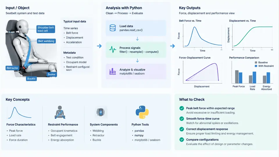
Seatbelt force and restraint performance analysis sits at the intersection of vehicle crash dynamics, occupant biomechanics, and data engineering. The goal is deceptively simple: understand how the forces transmitted through a seatbelt system evolve during a crash event, and whether those forces keep an occupant within survivable injury thresholds. In practice, this requires processing high-rate sensor data, reconstructing occupant kinematics, and comparing measured or simulated responses against regulatory and consumer-rating criteria. Python has become the de facto tool for this work because it combines fast numerical computation, mature signal-processing libraries, and a flexible ecosystem for visualization and reporting.
This course treats Python not as a general programming subject but as the working instrument of a restraint analyst. Every chapter is anchored to a real analysis task: loading crash-test channels, filtering accelerometer noise, computing belt-force time histories, deriving occupant displacement, and judging results against injury criteria such as HIC, chest deflection, and belt load limits. By the end, you should be able to take a raw test or simulation dataset and produce a defensible restraint performance assessment.
What "Seatbelt Force and Restraint Performance" Actually Means
A seatbelt system is a force-management device. During a frontal impact, the occupant continues moving forward while the vehicle decelerates. The belt converts that relative motion into a controlled deceleration by stretching, paying out through the retractor, and loading the occupant's skeletal structure at the pelvis and chest. The quantities that matter are therefore not just peak force but the shape of the force–time curve: how quickly load rises, how long it stays high, and how it is distributed between the lap and shoulder paths.
Three physical sub-systems interact:
- The belt and hardware — webbing stiffness, elongation, retractor lock-up, pretensioner firing, and load limiter (force limiter) behavior.
- The occupant — mass, seating posture, and the compliance of the chest and pelvis that determines how much force the body can tolerate.
- The vehicle — the crash pulse (deceleration history) that drives the entire event and the geometry of the seat and anchor points.
Restraint performance is the outcome of these three interacting. A stiff belt with no load limiter may produce very high chest loads; a soft belt may allow excessive forward excursion and contact with the steering wheel. Analysis exists to find the balance.
The Python Technical Context
The analysis workflow relies on a small, stable set of libraries. Understanding their roles early prevents the common mistake of reaching for the wrong tool.
| Library | Role in restraint analysis | Typical use |
|---|---|---|
| NumPy | Array math and time-base handling | Resampling, integration, unit conversion |
| pandas | Tabular channel data and metadata | Loading CSV/MDF channels, aligning signals |
| SciPy | Signal processing and filtering | Butterworth filters, CFC filtering, peak detection |
| Matplotlib | Time-history and criteria plots | Force–time curves, HIC windows, report figures |
Crash data is sampled at high rates — commonly 10 kHz for accelerometers and 10–20 kHz for belt load cells. At these rates, a one-second event contains tens of thousands of samples per channel. Python handles this comfortably, but the analyst must be disciplined about the time base: every channel must share a common, verified sample interval before any comparison or integration is attempted.
Coordinate and Sign Conventions
Before any calculation, fix the reference frame. In this course we adopt the standard vehicle crash convention:
- +X points forward (direction of travel).
- +Y points to the occupant's left.
- +Z points upward.
Accelerometer signals are typically recorded in g and must be converted to m/s² (multiply by 9.80665) before integration. Belt tension is recorded in newtons; a positive value means the belt is in tension. Because deceleration during a frontal crash is negative in the +X direction, a sled or vehicle pulse will appear as a negative acceleration. Keep this convention consistent across every chapter and every plot; a sign flip is one of the most common and most damaging analysis errors.
The Analysis Pipeline at a Glance
The figure below shows how raw measurements become a restraint performance judgment. It is a data-flow view, not a step-by-step procedure: each stage transforms one representation of the event into the next, and the feedback path shows that criteria evaluation often sends the analyst back to the filtering or alignment stage.
What You Will Be Able to Do
By the end of the course, the following capabilities define success. They are stated as observable outcomes rather than topics, because restraint analysis is judged by results, not by familiarity.
- Load a multi-channel crash dataset, verify its time base, and convert raw units into a consistent SI representation.
- Apply the correct filter class to each channel and justify the choice in terms of the physical bandwidth of interest.
- Compute belt force, occupant velocity, and forward excursion from acceleration and load-cell data, and explain each integration step.
- Evaluate injury criteria — HIC, chest deflection, and belt load limits — and interpret margin against the applicable threshold.
- Produce a clear, reproducible report figure set that another engineer can audit.
A Worked Orientation Example
To make the scope concrete, consider a simplified frontal sled case. A 78 kg occupant is restrained by a three-point belt with a load limiter set to approximately 4 kN. The sled pulse is a half-sine deceleration peaking near 40 g. The belt load cell records tension at 10 kHz. A minimal orientation script looks like this:
import numpy as np
import pandas as pd
from scipy.signal import butter, filtfilt

# Load one channel; assume columns: time_s, belt_force_N
df = pd.read_csv("sled_run_01.csv")
t = df["time_s"].to_numpy()
f_belt = df["belt_force_N"].to_numpy()

# Verify uniform sample interval before any processing
dt = np.diff(t)
assert np.allclose(dt, dt[0], atol=1e-9), "Non-uniform time base"
fs = 1.0 / dt[0]
print(f"Sample rate: {fs:.0f} Hz, samples: {len(t)}")

# CFC 60 low-pass filter (cutoff ~100 Hz) for belt force
b, a = butter(2, 100 / (fs / 2), btype="low")
f_filt = filtfilt(b, a, f_belt)

print(f"Peak belt force: {f_filt.max():.0f} N")
print(f"Time of peak:    {t[np.argmax(f_filt)]*1000:.1f} ms")
Running this on a representative dataset would print a sample rate near 10000 Hz, a peak belt force in the low-kilonewton range, and a peak time within the first 100 ms of the event. These are orientation values, not measured results; the point is that the entire analysis rests on three verifications — uniform time base, correct filter, and physically plausible peak. If the peak force appears at t = 0 or exceeds the load limiter setting by a large margin, the filter or the zero offset is wrong.
How the Course Is Organized
The chapters progress from data handling through signal conditioning, derived-quantity computation, criteria evaluation, and finally reporting and sensitivity studies. Each chapter builds on the previous one's outputs, so the scripts you write early become the foundation for later analysis. The emphasis throughout is on reproducibility: every number in a report should be traceable to a documented transformation of a named input channel.
Restraint performance analysis rewards precision. A filter chosen carelessly, a sign convention applied inconsistently, or an integration performed on a drifting signal will produce results that look plausible and are wrong. Python gives you the tools to do this work quickly; the discipline of verifying each stage is what makes the results trustworthy.