4. Signal conditioning
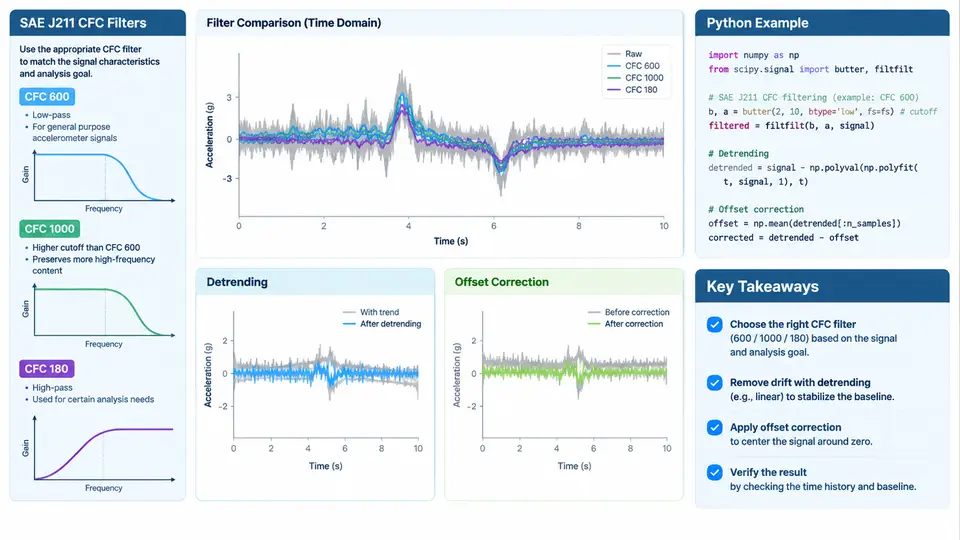
Raw data from accelerometers, load cells, and potentiometers in a crash test is never ready for injury-metric calculation the moment it leaves the DAQ. Before any HIC, chest deflection, or femur-load number can be trusted, the signal must pass through a deterministic conditioning chain defined by SAE J211/1. This chapter covers the three operations that dominate that chain in Python: low-pass filtering at CFC 600, 1000, and 180, detrending, and offset (zero) correction. Getting the order and parameters right is not cosmetic — a misapplied filter can shift peak acceleration by several percent and change a HIC15 value enough to flip a pass/fail decision.
Why CFC matters and where each class applies
SAE J211 defines Channel Frequency Class (CFC) as a fourth-order Butterworth low-pass characteristic with a specified −3 dB cutoff at fc = CFC × 0.6 (in Hz, with CFC expressed in the same units). The standard also fixes the tolerance band on the magnitude response and, critically, requires zero-phase filtering so that the time of the peak is not shifted. In practice this is achieved by applying the filter forward and then backward (filtfilt), which doubles the effective order and cancels phase.
| CFC | −3 dB cutoff fc | Typical channels |
|---|---|---|
| CFC 1000 | 600 Hz | Head CG accelerometers, upper-neck loads |
| CFC 600 | 360 Hz | Chest accelerometers, femur/tibia loads, pelvis |
| CFC 180 | 108 Hz | Chest deflection, belt force, occupant displacement |
The rule of thumb: the stiffer and more localized the structure being measured, the higher the CFC. Head acceleration contains energy well above 300 Hz, so CFC 1000 is mandatory; a chest potentiometer or belt load cell rarely carries meaningful content above 100 Hz, so CFC 180 removes noise without attenuating the physical response.
Implementing the J211 filter in Python
The cleanest approach is a small helper that builds the second-order Butterworth sections and applies them zero-phase. Because J211 specifies a fourth-order response, we design a 2nd-order Butterworth and run it forward-backward, giving an effective 4th-order magnitude with zero phase.
import numpy as np
from scipy.signal import butter, filtfilt

def j211_filter(signal, fs, cfc):
    """Zero-phase 4th-order Butterworth per SAE J211.
    fs  : sample rate [Hz]
    cfc : 600, 1000, or 180
    """
    fc = cfc * 0.6                      # -3 dB cutoff
    wn = fc / (fs / 2.0)                # normalized to Nyquist
    b, a = butter(2, wn, btype='low')   # 2nd order -> 4th after filtfilt
    return filtfilt(b, a, signal)

# example: head CG accel at 10 kHz, CFC 1000
a_filt = j211_filter(a_raw, fs=10000, cfc=1000)
Two practical cautions. First, filtfilt uses padding to reduce edge transients; the default padlen is 3 * max(len(a), len(b)), which is fine for long records but can fail on very short signals — pass an explicit padlen if you hit a ValueError. Second, always verify the cutoff: a quick check is to feed a sine sweep and confirm the −3 dB point lands at cfc × 0.6. If your sample rate is below roughly 5× the cutoff, the digital filter will deviate from the analog J211 template and the result is no longer compliant.
Offset correction
Offset correction removes the constant bias present before the event. The standard method is to compute the mean over a pre-trigger window — typically the 20–50 ms immediately preceding T0 — and subtract it from the entire record. This must be done on the raw signal, before filtering.
def remove_offset(signal, fs, t0_index, pre_ms=50):
    n = int(pre_ms * fs / 1000)
    start = max(0, t0_index - n)
    bias = np.mean(signal[start:t0_index])
    return signal - bias, bias
Choose the pre-trigger window carefully. If the vehicle is already moving or the channel shows drift before impact, a longer window captures the drift but a shorter one avoids it. For load cells, a 30 ms window ending 5 ms before T0 is a common compromise. Record the computed bias in your report — an unusually large value (e.g., > 5% of full scale) is a red flag for a sensor or cabling problem.
Detrending
Detrending removes low-frequency drift that offset correction cannot handle — thermal drift in a strain-gauge bridge, or slow baseline wander in an accelerometer. The standard practice is linear detrending over the pre-event window only, then applying that same linear correction across the whole record. Detrending the entire signal (including the crash pulse) would remove real physical content and is incorrect.
def detrend_pre_event(signal, fs, t0_index, pre_ms=50):
    n = int(pre_ms * fs / 1000)
    start = max(0, t0_index - n)
    seg = signal[start:t0_index]
    x = np.arange(len(seg))
    slope, intercept = np.polyfit(x, seg, 1)
    full_x = np.arange(len(signal)) - start
    return signal - (slope * full_x + intercept)
Apply detrending after offset correction and before filtering. The order is therefore: offset → detrend → filter. Reversing offset and detrend is harmless in most cases, but filtering before either will smear the bias into the event window and corrupt the peak.
Verifying the conditioned signal
After conditioning, run three checks before feeding the data into injury metrics. First, confirm the pre-trigger baseline is flat and centered on zero — a residual slope indicates detrending failed. Second, inspect the peak: filtering should reduce the raw peak slightly (typically 1–5% for CFC 1000, more for CFC 180), never increase it. Third, compare the time of the peak before and after filtering; with zero-phase filtering it should not move by more than one sample. If the peak shifts noticeably, you have likely used a causal filter (lfilter) instead of filtfilt.
fs, cfc, the pre-trigger window length, and the computed bias alongside every conditioned channel. When a HIC value is questioned later, these four numbers let anyone reproduce the exact waveform.
A common failure mode is applying CFC 180 to a head accelerometer "to smooth it." This over-attenuates the high-frequency content that drives HIC and produces a falsely low value. Always match the CFC to the channel per the test protocol, and document the choice. With offset, detrend, and the correct J211 filter applied in the right order, the conditioned signal is ready for the injury-metric calculations that follow.