1. Course overview
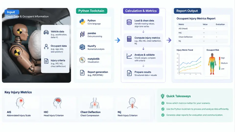
Crash safety engineering depends on a small set of scalar metrics that compress a complex, high-rate physical event into numbers a regulator, a program manager, or a design engineer can compare against a limit. The most familiar are HIC (Head Injury Criterion), a3ms (the 3 ms clip of the resultant chest acceleration), Nij (Neck Injury Criterion), and Dmax (chest deflection). Each is derived from filtered accelerometer or displacement channels recorded during a sled or full-vehicle test, and each has a defined time window, filter class, and pass/fail threshold. This chapter establishes the vocabulary, the software stack, and the pipeline that the remaining 29 chapters build on.
What the metrics actually are
HIC is defined over a window bounded by t1 and t2, with a maximum duration of 36 ms:
HIC = max over (t1, t2) of [ (t2 - t1) * ( (1/(t2-t1)) * ∫ a(t) dt )^2.5 ]
      subject to t2 - t1 ≤ 0.036 s
The acceleration a(t) is the resultant of the three head-CG channels, expressed in g, and is filtered per SAE J211 (typically CFC 1000 for head). The 2.5 exponent makes HIC disproportionately sensitive to short, high-amplitude spikes, which is why filter class and window search strategy matter as much as the raw data.
a3ms is simpler: compute the resultant chest acceleration, apply the CFC 180 filter, then slide a 3 ms window and take the maximum mean. Nij combines axial force and bending moment, each normalized by a critical intercept value, and is evaluated as the maximum of four combinations (tension-extension, tension-flexion, compression-extension, compression-flexion). Dmax is the peak chest deflection from a displacement sensor, filtered at CFC 180.
The Python toolchain
The reference stack for this course is deliberately small and reproducible:
- NumPy — array math, integration, windowed operations.
- SciPy —
scipy.signal.butterandsosfiltfiltfor zero-phase SAE J211 filtering. - pandas — channel tables, test metadata, and result aggregation across runs.
- iso13499 / in-house
injurypackage — reference implementations of HIC, Nij, and a3ms; used here as a cross-check, not a black box. - Matplotlib — time-history plots and window overlays for QC.
- Jinja2 + WeasyPrint — HTML/PDF report generation from a template.
- pytest — regression tests against known-answer fixtures.
Install with a pinned environment so results are reproducible across machines:
python -m venv .venv
source .venv/bin/activate
pip install numpy==1.26.4 scipy==1.13.0 pandas==2.2.2 \
            matplotlib==3.8.4 jinja2==3.1.4 weasyprint==61.2 pytest==8.2.0
The end-to-end workflow
The pipeline has five stages, and each stage has a failure mode that shows up as a plausible-but-wrong number rather than an exception. The diagram below shows the data flow and the QC checkpoint at each stage.
Stage 1 — Ingest and metadata
Test data arrives as ISO MME, DIAdem, or CSV exports. The critical step is not reading the file but binding each channel to its physical location and filter class. A minimal channel table looks like this:
channel_id, location, direction, unit, cfc, sample_rate_hz
HEAD_CG_X,  head_cg,  x,  g,  1000, 10000
HEAD_CG_Y,  head_cg,  y,  g,  1000, 10000
HEAD_CG_Z,  head_cg,  z,  g,  1000, 10000
CHEST_X,    chest,    x,  g,   180, 10000
CHEST_Y,    chest,    y,  g,   180, 10000
CHEST_Z,    chest,    z,  g,   180, 10000
CHEST_DEF,  chest,    y,  mm,  180, 10000
If the sample rate is not uniform, resample to a common grid before filtering. If t0 is not aligned across channels, the resultant computation will mix non-simultaneous samples and produce a physically impossible vector magnitude.
Stage 2 — Conditioning
SAE J211 filtering is a zero-phase, second-order Butterworth applied forward and backward. In SciPy:
from scipy.signal import butter, sosfiltfilt

def j211_filter(x, fs, cfc):
    # 3 dB cutoff at cfc; standard J211 uses a 2nd-order Butterworth
    sos = butter(2, cfc / (fs / 2.0), btype='low', output='sos')
    return sosfiltfilt(sos, x)
Two mistakes are common. First, using lfilter instead of sosfiltfilt introduces phase shift and inflates the peak. Second, applying the filter twice (once per channel, then again on the resultant) over-attenuates the signal. Filter each component once, then compute the resultant.
Stage 3 — Computation
For HIC, the window search is the expensive part. A vectorized approach using cumulative integration is standard:
import numpy as np

def hic(a_g, dt, max_window_s=0.036):
    # a_g: filtered resultant head acceleration in g
    n = len(a_g)
    max_n = int(max_window_s / dt)
    # cumulative integral of a
    cum = np.concatenate(([0.0], np.cumsum(a_g) * dt))
    best = 0.0
    best_t1 = best_t2 = 0
    for i in range(n):
        j_end = min(i + max_n, n)
        # mean acceleration over [i, j]
        for j in range(i + 1, j_end + 1):
            mean_a = (cum[j] - cum[i]) / ((j - i) * dt)
            hic_val = ((j - i) * dt) * (mean_a ** 2.5)
            if hic_val > best:
                best = hic_val
                best_t1, best_t2 = i, j
    return best, best_t1 * dt, best_t2 * dt
For a 10 kHz signal over 200 ms, the naive double loop is slow; in practice, use the standard optimization that fixes the window end and searches backward, or use numba/numpy vectorization. The result must always be reported with its t1 and t2, because a HIC value without a window is not auditable.
Stage 4 — Validation against limits
Typical limits used in this course (illustrative, not a substitute for the current regulation text):
| Metric | Typical limit | Filter | Window |
|---|---|---|---|
| HIC | 700 (FMVSS 208, 36 ms) | CFC 1000 | ≤ 36 ms |
| a3ms | 60 g | CFC 180 | 3 ms clip |
| Nij | 1.0 | CFC 600 | peak |
| Dmax | 63 mm | CFC 180 | peak |
Each computed value is compared to its limit and tagged PASS or FAIL. A margin column (limit - value) is more useful than the flag alone, because it shows how close the design is to the boundary.
Stage 5 — Reporting
The report is generated from a Jinja2 template that receives a results dictionary and a set of Matplotlib figures. The template renders a summary table, one time-history plot per metric with the critical window shaded, and a traceability block listing the input file hash, filter parameters, and code version. This is what makes the result defensible in a design review.
What you will build across this course
By the end of the 30 chapters, you will have a working Python package that ingests a channel table, applies the correct J211 filters, computes HIC, a3ms, Nij, and Dmax, validates them against a configurable limit set, and emits a PDF report with plots and traceability metadata. The package will be covered by pytest fixtures using synthetic signals with known analytical answers, so that every change to the filtering or window logic is caught before it reaches a report.
The first practical step is to set up the environment and load a sample channel table. The next chapter walks through that ingestion layer in detail, including how to handle missing channels, unit mismatches, and non-uniform sample rates without silently corrupting the downstream metrics.