4. Time synchronization and signal alignmen
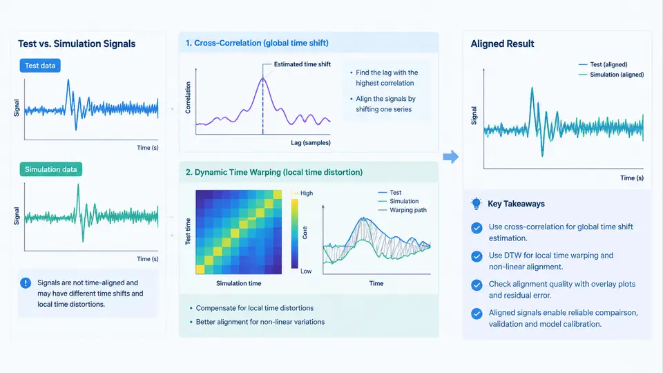
Before any meaningful correlation metric can be computed, the test and simulation signals must occupy the same time base. In crash test and simulation correlation work, this is rarely a matter of simply subtracting a constant offset. The two signals typically differ in three independent ways: a time offset (the simulation event starts at a different absolute time than the physical event), a time scale or rate mismatch (the simulated event unfolds slightly faster or slower than the physical one), and shape distortion (local stretching or compression caused by model stiffness errors, contact timing, or filtering differences). Cross-correlation addresses the first two; dynamic time warping (DTW) addresses the third. A robust workflow applies them in that order.
Why Raw Overlay Plots Mislead
A common failure mode is to plot the filtered test acceleration and the simulated acceleration on the same axis, observe a large peak-to-peak error, and conclude the model is wrong. In practice, a 3–8 ms timing shift on a 40 g pulse with a 10 ms rise time can produce an apparent amplitude error of 30% or more, even when the underlying pulse shapes are nearly identical. The correlation engineer must therefore separate timing error from amplitude error before attributing discrepancy to the model.
Step 1 — Establish a Common Reference and Sign Convention
Define the reference frame explicitly and keep it consistent throughout the analysis. In this chapter, positive time runs forward from the trigger instant, and the test signal is treated as the reference; the simulation is shifted to match the test. All lags reported are therefore "simulation lag relative to test." If the opposite convention is used, every reported lag changes sign — document the choice in the correlation report.
Both channels must also share a common sample rate before alignment. Resample the lower-rate channel onto the higher rate using a band-limited interpolator (e.g., scipy.signal.resample_poly or a zero-phase anti-alias filter followed by linear interpolation). Do not align signals at different sample rates by index.
Step 2 — Coarse Alignment by Cross-Correlation
The cross-correlation function R_xy(τ) measures the similarity between the test signal x(t) and the simulation signal y(t) as a function of lag τ. The lag at which R_xy peaks is the best global time shift under the assumption of a single rigid offset.
import numpy as np
from scipy.signal import correlate, correlation_lags

# x: test acceleration, y: simulation acceleration, both at fs = 10 kHz
x = x - x.mean()
y = y - y.mean()

corr = correlate(y, x, mode="full")
lags = correlation_lags(len(y), len(x), mode="full")
lag_samples = lags[np.argmax(corr)]
lag_ms = lag_samples / fs * 1000.0

# Apply the shift so that simulation aligns to test
y_aligned = np.roll(y, -lag_samples)
For a typical frontal rigid-barrier pulse sampled at 10 kHz, a peak at lag_samples = -35 means the simulation leads the test by 3.5 ms; rolling the simulation forward by 35 samples aligns the two dominant peaks. Always verify the peak is unambiguous — if the correlation function has two comparable peaks, the signal contains periodic content or the event window is too wide, and the coarse alignment is unreliable.
corr / (norm(x) * norm(y))) so the peak value can be read as a similarity coefficient between −1 and 1. A peak below roughly 0.7 on a clean crash pulse usually indicates a genuine shape mismatch, not a timing problem.Step 3 — Refine with Dynamic Time Warping
Cross-correlation assumes a single constant shift. Real crash signals violate this: the occupant kinematics may be well-timed at 20 ms but drift by 4 ms at 60 ms because the model's restraint stiffness is slightly off. DTW finds a non-linear warping path that maps the simulation time axis onto the test time axis, minimizing cumulative distance while respecting monotonicity and continuity constraints.
from dtaidistance import dtw
import numpy as np

# Downsample to 1 kHz for DTW; full 10 kHz is unnecessary and slow
x_ds = x[::10]
y_ds = y_aligned[::10]

# Sakoe-Chiba band limits warping to +/- 5 ms (5 samples at 1 kHz)
path = dtw.warping_path(x_ds, y_ds, window=5)
# path is a list of (test_index, sim_index) pairs
The window parameter is the critical control. A band that is too narrow prevents DTW from correcting real drift; a band that is too wide allows the algorithm to "cheat" by warping unrelated features into alignment, producing an artificially low residual. For crash pulses, a band of ±5 to ±10 ms is a practical starting point. Inspect the warping path: a nearly diagonal path means the signals were already well aligned; a path with visible steps or plateaus indicates localized timing distortion worth investigating in the model.
Step 4 — Validate the Alignment
Alignment is not complete until it is verified. Three checks are standard:
- Peak timing residual: after warping, the time difference between corresponding peaks (e.g., first acceleration peak, rebound peak) should be under 1–2 ms for a well-correlated model.
- Residual energy: compute the RMS of
x − y_warpedover the event window and compare it to the RMS ofx. A ratio above ~0.25 typically signals a shape problem that alignment cannot fix. - Warping path smoothness: a path with large local slope changes means the time mapping is unstable; report the maximum local slope as a quality indicator.
Choosing Between the Two Methods
| Condition | Recommended method | Reason |
|---|---|---|
| Single dominant pulse, uniform timing error | Cross-correlation only | One rigid shift is sufficient; DTW adds risk without benefit |
| Multi-phase event (compression, rebound, secondary impact) | Cross-correlation, then banded DTW | Phase-dependent drift requires non-linear mapping |
| Signals with strong periodic content (e.g., belt rattle) | Cross-correlation with caution; avoid DTW | Periodicity creates ambiguous correlation peaks and unstable warping |
| Very noisy low-amplitude channels | Low-pass filter first, then cross-correlation | Noise dominates the distance metric and corrupts both methods |
Worked Example: Frontal Pulse Alignment
Consider a 50 km/h frontal rigid-barrier test with a chest acceleration channel sampled at 10 kHz. The raw simulation leads the test by an unknown amount. Cross-correlation returns a peak at −3.5 ms with a normalized coefficient of 0.91, indicating a strong global match. After shifting, the first peak aligns within 0.4 ms, but the rebound peak at 85 ms still shows a 3 ms lead. Applying banded DTW with a ±8 ms window reduces the rebound residual to 0.9 ms and lowers the residual RMS ratio from 0.31 to 0.18. The warping path is smooth except for a small step near 60 ms, which points to a restraint locking timing difference — a specific, actionable finding for the modeler.
Practical Notes on Filtering and Windowing
Both cross-correlation and DTW operate on the signal you give them, so the preprocessing choice matters as much as the algorithm. Apply the same anti-alias filter (typically a 4th-order Butterworth low-pass at 1–2 kHz for crash accelerometers, per SAE J211 channel class) to both channels before alignment. If the test channel is filtered at 1000 Hz and the simulation at 2000 Hz, the cross-correlation peak will be biased toward the sharper signal. Also restrict the analysis window to the event of interest — including pre-trigger idle data adds flat regions that can pull the correlation peak toward zero lag.
Finally, record the alignment parameters in the correlation report: the lag applied, the DTW window, the sample rate used, and the filter settings. Without these, a reviewer cannot reproduce the alignment, and the correlation coefficient becomes an unverifiable number. Alignment is a preprocessing decision, not a cosmetic adjustment, and it must be documented with the same rigor as the model itself.