1. Crash test and simulation data correlati
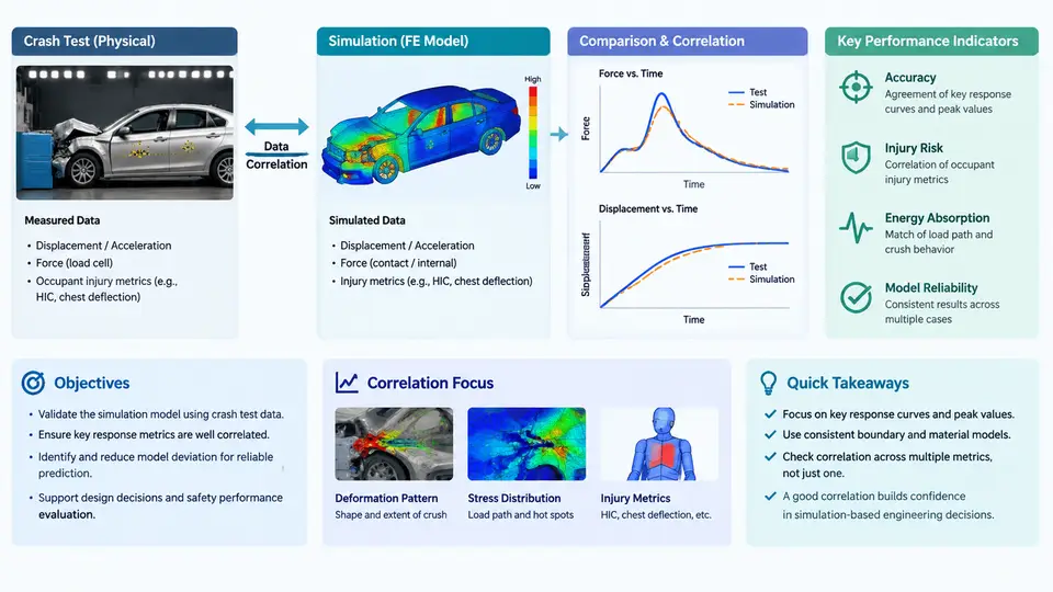
In vehicle safety engineering, a physical crash test and its corresponding CAE (Computer-Aided Engineering) simulation are two representations of the same event. The physical test produces measured responses from instrumented dummies, accelerometers, and high-speed video; the simulation produces predicted responses from an explicit finite element model solved in a code such as LS-DYNA or PAM-CRASH. Data correlation is the disciplined process of quantifying how well those two representations agree, explaining where they diverge, and deciding whether the model is trustworthy enough to support design decisions. It is not a cosmetic exercise in matching curves — it is the evidence base that allows engineers to replace expensive hardware iterations with validated virtual ones.
Why Correlation Matters
A frontal offset deformable barrier (ODB) test at 64 km/h consumes a full vehicle, a calibrated dummy, a barrier face, and several weeks of preparation. A validated model can run the same event overnight and then be used to sweep restraint parameters, barrier stiffness, or structural gauges that would never be affordable physically. The value of the model therefore depends entirely on demonstrated fidelity. Regulatory and consumer programs reinforce this: Euro NCAP and NHTSA increasingly accept simulation evidence for certain assessments, but only when the model has been correlated against physical tests with documented metrics and tolerances.
Correlation also serves a diagnostic purpose. When a simulation over-predicts chest deflection by 15 mm, the discrepancy points to a specific modelling assumption — belt stiffness, seat cushion friction, or dummy thorax material — that must be investigated. The correlation process converts a vague "the model looks wrong" into a traceable engineering question.
The Correlation Workflow
A defensible correlation study follows a repeatable sequence. The order matters because each stage constrains the next.
- Define the correlation matrix. Identify which physical tests will be correlated, which signals will be compared, and at which locations. A typical frontal ODB matrix includes vehicle CG accelerations (X, Y, Z), B-pillar and rocker accelerations, seat track accelerations, steering column displacement, belt force at the retractor and anchor, and dummy responses (head resultant acceleration, chest deflection, femur loads).
- Condition the measured data. Physical signals are filtered and resampled before comparison. The standard practice is to apply the same channel frequency class (CFC) filter to both test and simulation data — for example, CFC 60 for occupant accelerations and CFC 180 for structural accelerations per SAE J211. Without identical filtering, any metric comparison is meaningless.
- Align the time base. Test and simulation rarely share a common t=0. The conventional reference is the moment of first contact between the vehicle and the barrier, or a defined trigger such as a 0.5 g longitudinal acceleration threshold. A residual time shift of even 2–3 ms can dominate a cross-correlation score, so alignment is performed before any metric is computed.
- Compute quantitative metrics. Several complementary metrics are used because each captures a different aspect of agreement.
- Diagnose and iterate. Where metrics fall outside tolerance, the engineer traces the discrepancy to model inputs — material cards, contact definitions, joint stiffness, mass distribution — and updates the model. Each iteration is documented so the correlation history is auditable.
- Report and gate. The final correlation report states which signals pass, which are marginal, and which are accepted with justification. This report becomes the model's qualification record.
Key Performance Indicators
Correlation metrics fall into three families: magnitude, phase, and shape. Relying on any single metric invites false confidence.
| Metric | What it measures | Typical acceptance |
|---|---|---|
| Peak value ratio | Simulation peak ÷ test peak | 0.85–1.15 for structural channels |
| Time of peak difference | Phase alignment at the peak | ≤ 5 ms for structural, ≤ 10 ms for occupant |
| Cross-correlation coefficient (CCC) | Overall shape and phase agreement | ≥ 0.85 good, ≥ 0.70 marginal |
| Integrated absolute error (IAE) | Area between curves, normalized | ≤ 15% of test integral |
| Peak magnitude error | Absolute difference at peak | ≤ 10% of test peak |
The cross-correlation coefficient is computed as the maximum of the normalized cross-correlation function over a small time-shift window (typically ±5 ms). This window accommodates minor timing differences without rewarding gross misalignment. A high CCC with a poor peak ratio indicates the model captures the event's character but not its severity — a common signature of incorrect material strain-rate sensitivity.
Signal Chain and Data Flow
The correlation process is best understood as a signal chain in which each stage transforms the data and where errors can be introduced. The diagram below shows the parallel paths from physical test and simulation to the comparison stage, including the conditioning steps that must be identical on both sides.
Practical Considerations and Common Pitfalls
Several failure modes recur in correlation studies. First, filter mismatch: applying CFC 60 to the test but leaving the simulation unfiltered produces artificially high-frequency content that destroys the CCC. Second, mass and inertia discrepancies: a 2% difference in total vehicle mass or a misplaced battery pack shifts the entire acceleration history. Third, contact definition errors: missing or overly stiff contact between the dummy and seat can change chest deflection by more than 10 mm. Fourth, time-zero ambiguity: using the barrier trigger for the vehicle but the accelerometer threshold for the dummy introduces a systematic phase error.
What Good Correlation Looks Like
A well-correlated model does not match every signal perfectly. It matches the signals that matter for the intended application within documented tolerances, and it fails in explainable ways elsewhere. For a frontal restraint design study, the critical channels are occupant chest deflection, head acceleration, and belt forces; structural accelerations are secondary. The correlation report should therefore prioritize these channels and state explicitly which signals were used for model tuning and which were held back as validation channels. This separation — tuning set versus validation set — is what distinguishes a credible correlation from a curve-fitting exercise.
The ultimate test of correlation quality is predictive capability. After the model is correlated to a 64 km/h ODB test, it should be used to predict a 56 km/h or 72 km/h event without further tuning. If the prediction falls within the same tolerances, the model has genuine predictive value. If it does not, the correlation was likely over-fitted, and the underlying modelling assumptions need re-examination.