4. Data cleaning and transformation for CAE
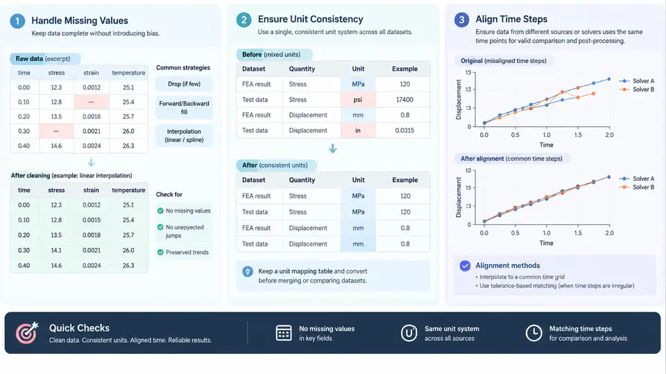
Raw solver output is rarely dashboard-ready. A transient structural run may write nodal displacement at every converged increment, a thermal solver may emit temperature on a coarse mesh, and a CFD post-processor may export surface pressure at irregular physical times. Before any chart, KPI tile, or report table can be trusted, the dataset must pass through a deterministic cleaning and transformation stage. This chapter focuses on three recurring problems in CAE result pipelines: missing values, unit consistency, and time-step alignment. The goal is not to make data "look nice" but to make it numerically defensible — every interpolation, fill, or conversion must be traceable and reversible.
Why CAE data is structurally messy
Unlike business datasets, CAE results carry physical meaning that constrains how they may be repaired. A missing von Mises stress value at a node is not equivalent to a missing customer age. It may indicate a non-converged increment, a deleted element, a rigid-body constraint, or a post-processor export gap. Treating all three as the same "NaN" and filling them with a column mean silently corrupts the field. The first discipline is therefore classification before correction: distinguish between structurally absent values (the quantity does not exist at that location), computationally missing values (the solver failed or skipped), and export-missing values (the value exists but was not written).
A practical way to encode this is a companion status column alongside each physical field. For example, a displacement table might carry U_mag plus U_mag_status with values such as ok, not_converged, inactive, and export_gap. Downstream aggregation can then decide policy per status rather than per NaN.
Handling missing values without falsifying physics
Three policies cover most CAE cases, and the choice should be driven by the physical role of the field:
- Drop — remove the record when the missing value is essential and cannot be reconstructed. Appropriate for a peak stress sample at a non-converged increment.
- Interpolate — reconstruct along a known axis (time, load step, or spatial coordinate) when the field is smooth and the gap is small. Appropriate for a temperature history with one dropped frame.
- Mark and propagate — keep the record but carry the status flag so that any aggregate (max, mean, percentile) can report coverage. Appropriate when the dashboard must show data availability honestly.
Linear interpolation in time is the most common repair. Given samples at t0 and t2 with a gap at t1, the reconstructed value is v1 = v0 + (v2 - v0) * (t1 - t0) / (t2 - t0). This is only valid if the underlying response is approximately linear over that interval. For oscillatory responses — modal, transient dynamic, or flutter — linear fill can attenuate peaks. In those cases, either drop the gap or use a shape-preserving method such as PCHIP, and always record the method in the dataset metadata.
Unit consistency across solvers and post-processors
CAE pipelines frequently mix unit systems. A Nastran deck may use mm–N–MPa, an Abaqus input may use m–N–Pa, and a CFD export may use mm–s–kg. When these streams meet in one dashboard, a displacement of 2.5 is meaningless until its unit is known. The robust approach is to normalize everything to a single canonical unit system at ingestion, and to store the original unit as metadata.
A minimal canonical set for structural and thermal dashboards is: length in mm, force in N, stress in MPa, mass in tonne, time in s, temperature in °C. Conversion factors are then applied as pure multipliers, and derived quantities must be converted with the correct exponent. Stress, for example, scales with the square of the length factor when force is held fixed, while density scales with mass divided by length cubed.
| Quantity | Source unit | Canonical unit | Factor |
|---|---|---|---|
| Length | m | mm | × 1000 |
| Force | kN | N | × 1000 |
| Stress | Pa | MPa | × 1e-6 |
| Density | kg/m³ | tonne/mm³ | × 1e-12 |
| Temperature | K | °C | − 273.15 |
Temperature is the exception that breaks the pure-multiplier rule because it has an offset. Any pipeline that stores a single "scale" per field will silently corrupt Kelvin-to-Celsius conversions. Store both scale and offset, and apply canonical = raw * scale + offset uniformly.
Time-step alignment across result streams
Transient CAE results are the hardest case because different solvers advance time differently. An implicit structural solver may output at adaptive increments (0.01 s, 0.013 s, 0.021 s …), while an explicit crash solver outputs at fixed small steps, and an experimental measurement may sample at 100 Hz. To compare or overlay these streams, they must be resampled onto a common time base.
The recommended procedure is:
- Define a target time vector — either the union of all timestamps, or a uniform grid at a resolution finer than the coarsest stream.
- For each stream, interpolate onto the target vector using a method appropriate to the physics (linear for quasi-static, PCHIP or spline for smooth dynamic, zero-order hold for discrete events).
- Record, per target time, which streams were interpolated versus directly sampled. This distinction matters when reporting peak values.
- Reject alignment when the extrapolation distance exceeds a tolerance — for example, do not extrapolate more than one source step beyond the last sample.
A subtle but important point: aligning time steps changes the effective sampling of peak quantities. If a structural stream peaks at t = 0.017 s but the target grid is 0.01 s, the peak will be missed unless the grid is refined or the peak is carried forward as a separate annotation. Dashboards that show "max stress over time" must therefore either use the native peak or explicitly state the resampling resolution.
A reproducible cleaning recipe
The following Python fragment illustrates the three stages on a small synthetic dataset. It is intentionally minimal so that the logic is visible; in production, each stage would be a separate function with logging and schema validation.
import numpy as np
import pandas as pd

# --- Stage 1: classify missing values ---
df = pd.DataFrame({
    "t":      [0.010, 0.013, 0.021, 0.034, 0.048],
    "stress": [210.0, np.nan, 245.0, 260.0, np.nan],
    "status": ["ok", "not_converged", "ok", "ok", "export_gap"],
})

# Only interpolate export gaps; keep not_converged as NaN
df["stress_clean"] = df["stress"].copy()
gap_mask = df["status"] == "export_gap"
df.loc[gap_mask, "stress_clean"] = np.nan
df["stress_clean"] = df["stress_clean"].interpolate(method="linear")

# --- Stage 2: unit normalization (Pa -> MPa) ---
df["stress_MPa"] = df["stress_clean"] * 1e-6

# --- Stage 3: align to a uniform 0.005 s grid ---
target_t = np.arange(0.010, 0.048 + 1e-9, 0.005)
aligned = pd.DataFrame({"t": target_t})
aligned["stress_MPa"] = np.interp(target_t, df["t"], df["stress_MPa"])
aligned["sampled"] = aligned["t"].isin(df["t"])
After this pipeline, aligned contains a uniform time base, a normalized stress field in MPa, and a boolean sampled column that tells the dashboard whether each point was measured or interpolated. A KPI tile showing "peak stress" can then be computed only over sampled == True rows, or over all rows with an explicit note that interpolation was used.
Verification and common failure symptoms
Cleaning is only trustworthy if it is verified. Three checks catch most defects:
- Unit sanity — compare a known reference value (e.g., a hand-calculated tip deflection) against the normalized dataset. A factor-of-1000 error usually means a missing length or stress conversion.
- Coverage report — count rows per status flag. If
not_convergedexceeds a few percent, the underlying simulation, not the cleaning, is the problem. - Peak preservation — compare the maximum of the aligned series against the maximum of the raw series. A drop larger than the interpolation tolerance indicates the target grid is too coarse.
Typical failure symptoms and their causes: a dashboard showing physically impossible stress (unit mismatch), a time-history curve with flat plateaus (over-aggressive fill of non-converged increments), and a peak that shifts between runs (resampling grid not fixed). Each symptom points back to a specific stage, which is why the pipeline should be modular and each stage independently testable.
With missing values classified, units normalized to a canonical system, and all streams resampled onto a shared time base, the dataset is finally in a state where aggregation, charting, and reporting can proceed without hidden assumptions. The next stage of the dashboard — computing KPIs and rendering them — depends entirely on the integrity established here.