4. Response Surface Methodology (RSM)
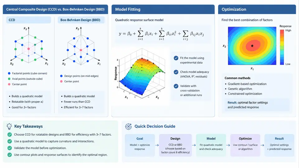
Response Surface Methodology (RSM) is a statistical and mathematical technique for building an approximate surrogate model of a CAE response when the underlying simulation is expensive to evaluate. Instead of running thousands of Monte Carlo samples, RSM fits a smooth polynomial surface to a carefully chosen set of design points, then uses that surface for prediction, sensitivity analysis, and optimization. In CAE workflows, RSM is most valuable when the design space is moderate in size (typically 2–8 factors), the response is continuous, and the goal is to locate an optimum or map a feasible region rather than characterize highly nonlinear or discontinuous behavior.
Design Selection: CCD vs. Box-Behnken
Two classical RSM designs dominate CAE practice: the Central Composite Design (CCD) and the Box-Behnken Design (BBD). Both fit a full quadratic model, but they differ in point placement, run count, and suitability for different factor constraints.
A CCD consists of three parts: a factorial (or fractional factorial) core at ±1 levels, axial (star) points at ±α on each axis, and center points. The value of α determines the design's rotatability. For a rotatable CCD with k factors, α = (2k)1/4. For k = 3, α ≈ 1.682. A CCD with k = 3 and a full factorial core has 23 + 2·3 + nc runs; with 6 center points, that is 8 + 6 + 6 = 20 runs. CCDs are sequential: you can start with a factorial, add axial points later, and reuse earlier runs.
A Box-Behnken design places points at the midpoints of edges of the factor space, never at the corners. For k = 3, a BBD has 12 edge points plus center points, typically 15–17 runs. BBDs avoid extreme corner combinations, which is advantageous when those corners are infeasible or physically unsafe. However, BBDs cannot be built for k = 2, and they do not support sequential augmentation as naturally as CCDs.
| Property | Central Composite (CCD) | Box-Behnken (BBD) |
|---|---|---|
| Factor levels | 5 (−α, −1, 0, +1, +α) | 3 (−1, 0, +1) |
| Runs (k = 3, 6 centers) | 20 | 15–17 |
| Corner points | Yes (factorial core) | No |
| Sequential augmentation | Excellent | Limited |
| Best when | Corners are feasible; rotatability needed | Corners infeasible; fewer runs desired |
In CAE, the choice often hinges on physical feasibility. For example, if a crash simulation cannot tolerate simultaneous maximum thickness and minimum rib spacing, a BBD avoids those corner combinations. If the design space is a safe box and you want a rotatable surface, use a CCD.
Model Fitting and Diagnostics
After running the CAE solver at each design point, you fit a second-order polynomial:
y = β₀ + Σ βᵢxᵢ + Σ βᵢᵢxᵢ² + ΣΣ βᵢⱼxᵢxⱼ + εwhere xᵢ are coded factor values (−α to +α), β are regression coefficients, and ε is residual error. In Python, this is typically done with statsmodels or scikit-learn:
import numpy as np
import statsmodels.api as sm
from sklearn.preprocessing import PolynomialFeatures

# X: (n_runs, k) coded factor matrix
# y: (n_runs,) CAE response (e.g., max stress)
poly = PolynomialFeatures(degree=2, include_bias=False)
X_poly = poly.fit_transform(X)
X_poly = sm.add_constant(X_poly)

model = sm.OLS(y, X_poly).fit()
print(model.summary())
Key diagnostics to inspect before trusting the surface:
- R² and adjusted R²: values above 0.90 are typical for well-behaved CAE responses; below 0.80 suggests the quadratic form is inadequate.
- Lack-of-fit test: if significant (p < 0.05), the model misses structure that higher-order terms or a different design could capture.
- Residual plots: residuals should be structureless and roughly normal. A funnel shape indicates heteroscedasticity; curvature indicates missing terms.
- Influential points: Cook's distance > 1 flags runs that disproportionately drive the fit. Re-examine those CAE runs for solver non-convergence or mesh issues.
Optimization on the Response Surface
Once the quadratic model is validated, optimization becomes cheap because evaluating the polynomial takes microseconds. You can use gradient-based methods, grid search, or global optimizers. A typical workflow:
- Define the objective (minimize mass, maximize stiffness) and constraints (stress ≤ allowable, displacement ≤ limit).
- Use the fitted model to predict responses over a fine grid or via
scipy.optimize.minimize. - Verify the predicted optimum with a confirmatory CAE run.
- If the confirmatory result deviates significantly, augment the design with the new point and refit.
from scipy.optimize import minimize

def objective(x):
    x_poly = poly.transform(x.reshape(1, -1))
    x_poly = sm.add_constant(x_poly, has_constant='add')
    return model.predict(x_poly)[0]

bounds = [(-1.682, 1.682)] * k
res = minimize(objective, x0=np.zeros(k), bounds=bounds, method='L-BFGS-B')
print(res.x, res.fun)
The confirmatory run is essential. In structural CAE, the surrogate may predict a 12% mass reduction at a stress level just below yield, but the actual simulation could show stress 5% above yield due to nonlinear contact or plasticity not captured by the quadratic. Treat the RSM optimum as a candidate, not a final answer.
Practical CAE Example: Bracket Thickness Optimization
Consider a steel bracket with three design variables: thickness t (2–6 mm), fillet radius r (3–10 mm), and rib height h (5–20 mm). The response is maximum von Mises stress under a 500 N load. A BBD with 15 runs is chosen because the corner combination of maximum thickness and minimum fillet is known to cause mesh distortion.
After fitting the quadratic model, the significant terms are t, r, t·r, and t². The optimized coded values are t = −0.8, r = +1.2, h = +0.3, predicting a stress of 210 MPa. A confirmatory run gives 218 MPa, within 4% of prediction. The design is accepted because the allowable is 235 MPa.
When RSM Is Not Enough
RSM assumes a smooth, low-order polynomial relationship. In CAE, this assumption breaks down for:
- Highly nonlinear responses such as buckling or contact status changes, where a quadratic cannot capture abrupt transitions.
- Discontinuous or noisy outputs from adaptive remeshing or solver tolerance variations.
- High-dimensional spaces (k > 10), where the number of quadratic terms grows as k(k+1)/2 and the required runs become impractical.
In these cases, consider Kriging/Gaussian process models, radial basis functions, or polynomial chaos expansion. RSM remains an excellent first surrogate because it is transparent, fast to fit, and provides explicit coefficient-based sensitivity information.
The next step after RSM is often sensitivity analysis: using the fitted coefficients or variance decomposition to rank which factors most influence the response. That is the subject of the following chapter.