4. Time-series preprocessing for accelerati
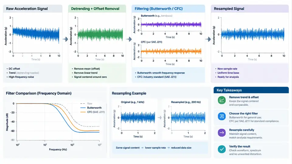
Raw acceleration data from a crash test or drop tower is never ready for direct analysis. A typical piezoelectric or piezoresistive accelerometer produces a voltage that is digitized by a data acquisition system, and what arrives in your Python session is a sequence of numbers contaminated by sensor offset, thermal drift, electrical noise, and a sample rate that may not match the rate required by the analysis standard. Before you can compute peak deceleration, injury criteria, or frequency content, you must condition the signal. This chapter covers the four preprocessing operations that matter most: offset removal, detrending, low-pass filtering with Butterworth and SAE J211 CFC filters, and resampling.
Why Preprocessing Is Not Optional
Consider a 50 g frontal impact pulse recorded at 10 kHz. The accelerometer may have a DC offset of 0.15 V, which after scaling becomes a constant 2 g bias. If you integrate that biased signal to get velocity, the bias accumulates linearly and the final velocity will be wrong by hundreds of mm/s. If you differentiate it to get jerk, the bias disappears but high-frequency noise is amplified catastrophically. If you compute a spectrum without filtering, aliased noise above the Nyquist frequency folds back into the band of interest and corrupts the result. Each preprocessing step addresses a specific failure mode, and skipping any one of them produces results that look plausible but are quantitatively wrong.
Offset Removal and Detrending
Offset removal subtracts a constant from the entire record. The standard approach is to compute the mean of a pre-trigger window — typically 50 to 100 ms of data before the impact event — and subtract that mean from every sample. This assumes the sensor was at rest during the pre-trigger window, which is almost always true in a controlled test.
import numpy as np

# accel: 1D array of acceleration in g
# fs: sample rate in Hz
# t_zero: time of impact trigger in seconds

pre_samples = int(0.100 * fs)          # 100 ms pre-trigger
trigger_idx = int(t_zero * fs)
baseline = np.mean(accel[trigger_idx - pre_samples:trigger_idx])
accel_zeroed = accel - baseline
Detrending goes further: it removes a linear trend, not just a constant. This is necessary when the sensor exhibits thermal drift during a long record, or when the pre-trigger window itself is not flat. In Python, scipy.signal.detrend with type='linear' fits and subtracts a least-squares line. For crash pulses, linear detrending is usually applied only when a constant offset removal leaves a visible slope in the pre-trigger region. Over-detrending can remove genuine low-frequency content from the pulse itself, so inspect the pre-trigger window before deciding.
Filtering: Butterworth vs. SAE J211 CFC
Filtering removes frequency content above the band of interest. Two filter families dominate acceleration signal processing: the Butterworth filter and the SAE J211 Channel Filter Class (CFC) filter.
A Butterworth low-pass filter is defined by its order and cutoff frequency. It has a maximally flat passband and a monotonic roll-off of 20·N dB per decade, where N is the order. In Python, scipy.signal.butter designs the coefficients and scipy.signal.sosfiltfilt applies them with zero phase distortion by filtering forward and backward. Zero-phase filtering is critical for crash pulses because phase distortion shifts the peak in time, which changes the timing of injury criteria.
from scipy.signal import butter, sosfiltfilt

def butter_lowpass(data, fs, cutoff, order=4):
    sos = butter(order, cutoff, btype='low', fs=fs, output='sos')
    return sosfiltfilt(sos, data)

accel_filt = butter_lowpass(accel_zeroed, fs=10000, cutoff=1650, order=4)
The SAE J211 standard specifies a different filter: the CFC filter, which is a fourth-order phaseless Butterworth filter with a defined cutoff frequency for each channel class. CFC 60 has a cutoff of 100 Hz, CFC 180 has 300 Hz, CFC 600 has 1000 Hz, and CFC 1000 has 1650 Hz. The standard also defines a tolerance corridor for the filter magnitude response, so a generic Butterworth design is not automatically J211-compliant unless it matches the specified cutoff and order.
| CFC Class | Cutoff Frequency (−3 dB) | Typical Use |
|---|---|---|
| CFC 60 | 100 Hz | Head, chest, pelvis acceleration |
| CFC 180 | 300 Hz | Dummy chest, femur |
| CFC 600 | 1000 Hz | Structural acceleration, component tests |
| CFC 1000 | 1650 Hz | High-frequency component response |
When implementing a CFC filter in Python, use a fourth-order Butterworth with the cutoff from the table and apply it with sosfiltfilt. The J211 tolerance corridor is checked by computing the magnitude response of the designed filter and comparing it to the standard's limits at defined frequencies. For most analysis work, matching the cutoff and order is sufficient; for certification testing, verify the response explicitly.
Resampling
Resampling changes the sample rate of a signal. It is needed when the acquisition rate differs from the analysis rate, when combining channels recorded at different rates, or when reducing data volume for storage. Two operations are involved: downsampling (decimation) and upsampling (interpolation).
Downsampling without prior anti-aliasing is dangerous. If you decimate a 10 kHz signal to 1 kHz by simply taking every tenth sample, any content between 500 Hz and 5 kHz folds back into the 0–500 Hz band. The correct procedure is to low-pass filter at the new Nyquist frequency first, then decimate. In Python, scipy.signal.resample_poly handles both the filtering and the rate change in one step using polyphase filtering.
from scipy.signal import resample_poly

# Downsample from 10 kHz to 1 kHz (factor 10)
accel_1k = resample_poly(accel_filt, up=1, down=10)

# Upsample from 1 kHz to 10 kHz (factor 10)
accel_10k = resample_poly(accel_1k, up=10, down=1)
For crash pulse analysis, resampling is often used to bring all channels to a common rate before computing relative displacements or injury criteria. The choice of rate depends on the highest frequency of interest: for CFC 600, a rate of at least 10 kHz is typical; for CFC 60, 1 kHz is sufficient.
Putting It Together: A Preprocessing Pipeline
The order of operations matters. A robust pipeline for a single acceleration channel is:
- Load raw voltage and apply the calibration factor to get acceleration in g.
- Remove offset using the pre-trigger mean.
- Apply linear detrending only if the pre-trigger window shows a slope.
- Apply the appropriate CFC or Butterworth low-pass filter with zero-phase filtering.
- Resample to the analysis rate if needed, using polyphase filtering.
- Verify: check that the pre-trigger mean is near zero, that the filtered peak is not attenuated below the expected value, and that the resampled signal preserves the pulse shape.
The verification step is where most preprocessing errors are caught. A common failure symptom is a filtered peak that is 10–20% lower than the unfiltered peak; this usually means the cutoff frequency is too low for the pulse content. Another symptom is a pre-trigger mean that drifts after filtering; this indicates that the filter's transient response has not settled, which happens when the pre-trigger window is shorter than the filter's impulse response. For a fourth-order Butterworth at 1650 Hz, the impulse response settles within roughly 2–3 ms, so a 100 ms pre-trigger window is more than sufficient. If you see drift, check that you are using sosfiltfilt and not sosfilt, and that the pre-trigger window is long enough.
Resampling artifacts are subtler. If you downsample without anti-aliasing, the pulse peak may shift or develop a ringing tail. If you upsample without proper interpolation, the pulse may appear jagged. Polyphase resampling with resample_poly avoids both problems because it applies an anti-aliasing filter as part of the rate conversion. Always compare the resampled signal against the original at the original rate to confirm that the peak value and pulse duration are preserved.