1. Crash pulse fundamentals and acceleratio
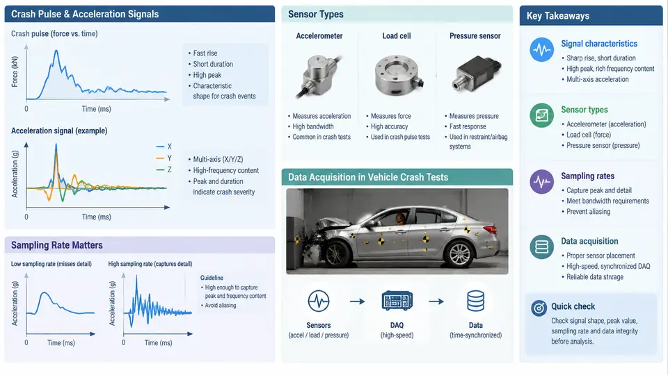
A crash pulse is the time history of vehicle deceleration (or acceleration) measured at a specific location on the vehicle body during an impact event. It is the single most important signal in vehicle crash testing because it encodes how the occupant compartment decelerates, how restraint systems load the occupants, and how structural crush energy is absorbed. In Python-based crash pulse analysis, everything downstream — filtering, integration, injury criteria, and pulse shaping — depends on correctly understanding what the sensor actually measures and how the data acquisition chain conditions that measurement.
Signal Characteristics of a Crash Pulse
A typical frontal rigid-barrier crash pulse lasts 80–150 ms. The vehicle starts at a defined impact velocity (for example, 56 km/h or 64 km/h in regulatory and consumer tests) and decelerates to zero. The acceleration signal is expressed in g (1 g = 9.80665 m/s²) and is conventionally signed so that deceleration during a frontal impact is negative when the sensor's positive axis points forward. This sign convention must be fixed before any integration, because velocity and displacement are obtained by cumulative integration of the acceleration signal.
Three features dominate the pulse shape:
- Rise time and peak — the initial slope and the maximum deceleration magnitude. A stiff structure produces a short, high-amplitude pulse; a compliant structure produces a longer, lower-amplitude pulse.
- Duration — the time from impact to the point where the vehicle has essentially stopped. It correlates with crush distance and available ride-down.
- Oscillatory content — high-frequency ringing from structural resonances, sensor mounting, and the barrier itself. This content is not occupant-relevant and must be removed by filtering.
The occupant-relevant frequency band is generally below 100–300 Hz. ISO 6487 and SAE J211 define the channel filter classes used in crash testing: CFC 60 (cut-off 100 Hz) for occupant acceleration, CFC 180 (cut-off 300 Hz) for structural acceleration, and CFC 1000 for high-bandwidth measurements. Applying the wrong filter class changes peak values and integrated velocity, so the filter class must be recorded with the channel.
Sensor Types and Mounting
Crash testing uses several accelerometer technologies:
| Sensor type | Typical range | Typical use | Notes |
|---|---|---|---|
| Piezoresistive (MEMS) | ±50 g to ±2000 g | Vehicle body, sled, barrier | DC response, good for integration; needs stable mounting |
| Piezoelectric (charge mode) | ±500 g to ±5000 g | High-shock structural points | No true DC response; charge amplifier required |
| Capacitive MEMS | ±50 g to ±500 g | Occupant and dummy channels | Integrated signal conditioning, common in onboard DAQ |
| Strain-gauge accelerometer | ±10 g to ±200 g | Low-g vehicle motion | Used where DC accuracy matters |
Mounting is as important as sensor selection. A sensor bolted to a flexible bracket will measure bracket resonance, not vehicle deceleration. The standard practice is to mount accelerometers on rigid structural members (B-pillar base, tunnel, sill, rocker) using machined blocks and short, stiff fasteners. The measurement axis must be aligned with the vehicle coordinate system: X forward, Y lateral, Z vertical, with the origin defined by the test protocol.
Sampling Rate and Anti-Alias Considerations
Sampling rate must be high enough to capture the highest frequency of interest and to allow digital filtering without aliasing. For CFC 180 channels, a minimum sample rate of 10 kHz is common; many labs use 20 kHz or higher to preserve margin. The Nyquist criterion requires fs > 2·fmax, but in practice a factor of 5–10 above the filter cut-off is used so that the anti-alias filter has a defined transition band.
Consider a channel filtered at CFC 180 (cut-off 300 Hz). Sampling at 10 kHz gives a Nyquist frequency of 5 kHz, which is more than 16× the cut-off. This is comfortable. Sampling at 1 kHz would give a Nyquist of 500 Hz — only 1.67× the cut-off — and any energy above 500 Hz would fold back into the passband. The result is a corrupted pulse that may show a false peak or a distorted rise time.
Data Acquisition Chain
A crash test data acquisition system typically consists of the following stages:
- Transducer — converts acceleration to an electrical signal (voltage, charge, or digital).
- Signal conditioning — amplifies, filters (anti-alias), and may provide excitation for piezoresistive bridges.
- Digitizer — samples the conditioned signal at the configured rate with a defined resolution (typically 16-bit or 24-bit).
- Onboard or offboard recorder — stores raw counts with time stamps and channel metadata.
- Calibration and scaling — converts counts to engineering units using the sensor's sensitivity and the channel gain.
The raw data is usually stored as counts. Scaling to g requires the sensitivity in mV/g, the amplifier gain, and the digitizer's volts-per-count. A typical scaling equation is:
acceleration_g = (raw_counts - zero_offset) * volts_per_count / (sensitivity_mV_per_g / 1000) / gainIf any of these terms is wrong, the pulse amplitude is wrong by a constant factor, and every integrated velocity and displacement will be wrong as well. This is why channel calibration records are part of the test documentation.
From Raw Signal to Analysis-Ready Pulse
The workflow from raw acquisition to an analysis-ready pulse is shown below. The key point is that filtering and zero-offset correction happen before integration, and the filter class is chosen from the measurement's intended use.
Practical Example: Scaling and First Inspection
Suppose a piezoresistive accelerometer with sensitivity 0.5 mV/g is connected to a channel with gain 100 and a 16-bit digitizer with a ±10 V range. The volts-per-count is 20 V / 65536 ≈ 305.2 µV/count. If the pre-impact zero offset is 32768 counts and the peak raw value during the crash is 41000 counts, the peak acceleration is:
delta_counts = 41000 - 32768 = 8232
voltage = 8232 * 305.2e-6 = 2.512 V
acceleration = 2.512 / (0.5e-3 * 100) = 50.2 g
This is a plausible peak for a CFC 180 structural channel in a moderate frontal impact. If the computed peak were 5 g or 500 g, the first things to check are the sensitivity value, the gain setting, and whether the zero offset was taken from a quiet window. A common failure symptom is a pulse that looks correct in shape but integrates to a final velocity far from the known impact velocity; this almost always indicates a scaling error or a DC offset drift.
What This Means for Python Analysis
When you load a crash pulse into Python, you are working with a scaled, filtered, time-aligned signal. The metadata that matters — sample rate, filter class, sensitivity, zero offset, sign convention, and channel location — must travel with the data. In the next chapters, we will use these signals for filtering, integration, pulse characterization, and occupant response analysis. The quality of every downstream result depends on getting the acquisition and conditioning right at this stage.