4. Extracting deployment time series
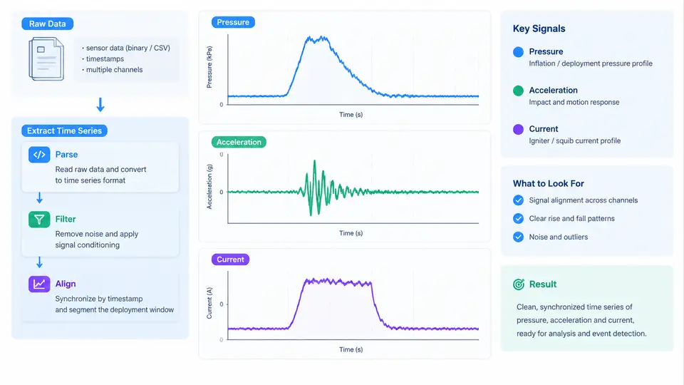
Raw airbag deployment logs rarely arrive as clean, aligned arrays. A typical bench or vehicle test produces several independent acquisition streams: a pressure transducer in the inflator plenum, one or more accelerometers on the steering-wheel hub or B-pillar, and a current shunt or Hall-effect sensor on the squib firing line. Each stream has its own sample rate, its own start trigger, and its own scaling. The task of this section is to turn those heterogeneous recordings into a single, time-aligned, physically meaningful set of series that later analysis stages can consume.
Before writing any extraction code, fix the reference conventions. We define t = 0 as the rising edge of the deployment command (the squib fire signal), positive acceleration as the direction of vehicle forward motion, and positive current as conventional current flowing from the firing circuit into the squib. Every downstream plot, threshold, and metric in this course inherits these definitions. If a dataset uses a different trigger or sign convention, convert it during extraction rather than patching it later.
What the raw data actually looks like
Most data acquisition systems export either a column-oriented CSV or a binary container (MDF4, TDMS, HDF5). A representative CSV export from a three-channel rig might look like this:
time_ms,pressure_kpa,accel_g,current_a
-2.000,101.3,0.002,0.000
-1.000,101.4,0.001,0.000
0.000,101.3,0.003,0.000
0.250,118.7,0.041,1.82
0.500,204.5,0.318,3.94
0.750,341.2,1.106,5.71
1.000,498.8,2.744,6.02
1.250,612.4,4.981,5.88
1.500,701.9,7.332,5.41
...
Three properties matter immediately. First, the channels are not guaranteed to share a time base — the pressure channel may be sampled at 10 kHz while the current channel runs at 50 kHz. Second, the trigger offset differs per channel because each logger arms independently. Third, the units are engineering units already scaled by the logger, but the scaling constants are often stored in a separate metadata block that must be applied explicitly.
Step 1 — Load and normalize the time base
Read each channel into its own array with its own native time vector. Do not assume a shared index. A robust loader keeps the raw time and value pairs together:
import numpy as np
import pandas as pd

def load_channel(path, t_col, v_col, t_scale=1e-3):
    df = pd.read_csv(path, usecols=[t_col, v_col])
    t = df[t_col].to_numpy(dtype=float) * t_scale   # ms -> s
    v = df[v_col].to_numpy(dtype=float)
    order = np.argsort(t)
    return t[order], v[order]
After loading, subtract the per-channel trigger time so that every channel's t=0 coincides with the fire command. If the logger records a dedicated trigger channel, detect its rising edge with a threshold crossing; otherwise use the first sample where the signal departs from its pre-trigger baseline by more than three standard deviations of the quiet region.
Step 2 — Resample onto a common grid
Analysis and cross-correlation require a single uniform time base. Choose a grid rate at or above the highest native rate to avoid aliasing; for airbag work, 20 kHz is a common compromise between fidelity and file size. Interpolate each channel onto that grid. Linear interpolation is acceptable for pressure and current; for acceleration, which contains high-frequency content, prefer a zero-phase filter followed by cubic interpolation, or resample in the frequency domain.
grid = np.arange(-0.002, 0.050, 1/20000)   # -2 ms to 50 ms

def resample(t, v, grid):
return np.interp(grid, t, v) # linear; use scipy.signal.resample for HFStep 3 — Apply calibration and unit conversion
Raw counts must be converted to engineering units using the calibration record shipped with the test. Pressure is typically reported in kPa or bar; acceleration in g; current in amperes. Apply the affine transform value = gain * raw + offset per channel, then convert to the course-standard units: kPa, g, and A. Record the calibration ID alongside the extracted series so results remain traceable.
Step 4 — Segment the deployment window
Extraction is not just alignment; it is also windowing. The interesting physics lives between the fire command and roughly 40–60 ms afterward. Define a pre-trigger baseline window (e.g., −5 ms to 0 ms) and a post-trigger analysis window (0 ms to 50 ms). Compute baseline statistics from the pre-trigger region and subtract the mean from each channel so that all signals start at zero. This baseline correction is essential for acceleration, where a small offset integrates into large velocity error.
The figure below shows how the three channels relate after extraction: the current pulse leads, pressure rises as the inflator generates gas, and acceleration responds once the bag contacts the occupant or the module reacts.
Step 5 — Validate the extraction
Before handing the series to analysis, run four checks. First, confirm that all channels share the same length and grid spacing. Second, verify that the pre-trigger baseline mean is within ±0.5% of the expected quiescent value (e.g., ~101.3 kPa for ambient pressure). Third, check that the current pulse integral — the charge delivered to the squib — falls within the manufacturer's specified range, typically 1.5–3.0 mC for a pyrotechnic initiator. Fourth, confirm that no channel contains NaN or clipped samples inside the analysis window.
| Check | Expected | Failure symptom | Likely cause |
|---|---|---|---|
| Grid alignment | Identical length & dt | Shape mismatch on concat | Different native rates not resampled |
| Baseline mean | Within ±0.5% of quiescent | Offset drift in acceleration | Missing baseline subtraction |
| Charge integral | 1.5–3.0 mC | Integral far below range | Current channel clipped or mis-scaled |
| Sample integrity | No NaN / clipping | Flat-top waveform | ADC saturation or dropped packet |
pressure, accel, current, plus a time dataset. This makes batch processing across hundreds of tests trivial and keeps calibration metadata attached.Common pitfalls and how to avoid them
The most frequent extraction error is applying a single time vector to channels that were logged independently. Always carry per-channel time arrays through the loading stage and only merge after resampling. The second most common error is forgetting that acceleration sign conventions differ between mounting orientations; a hub-mounted accelerometer may report negative g during bag deployment depending on its axis. Document the orientation in the metadata and, if necessary, flip the sign during extraction so that all tests share one convention.
A third pitfall is over-smoothing. It is tempting to apply a heavy low-pass filter to make plots look clean, but this destroys the peak acceleration value that later analysis depends on. Apply only the anti-aliasing filter required by the resampling step, and keep the raw series available for peak detection.
With the three channels extracted, aligned, calibrated, and validated, the next stage — computing deployment timing metrics such as time-to-first-pressure, peak acceleration, and charge duration — becomes a straightforward matter of indexing into a trustworthy array rather than wrestling with data plumbing.