1. Course overview
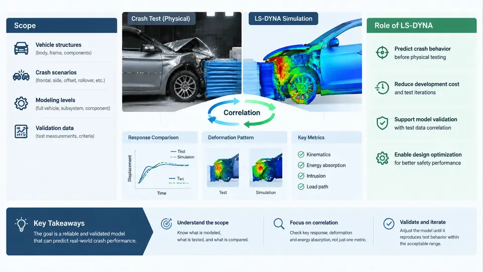
Vehicle crashworthiness development depends on a tight loop between physical testing and finite element simulation. A barrier impact test produces accelerometer traces, high-speed video, and deformation measurements; a CAE model produces the same quantities numerically. The engineering value of the model is determined entirely by how well those two sets of numbers agree — and by whether the disagreements can be explained, quantified, and reduced. This course is about that agreement, and about the disciplined process used to achieve it.
The scope of the course is correlation and validation, not model building from scratch. We assume you can already construct a full-vehicle LS-DYNA deck: mesh, materials, contacts, boundary conditions, and a stable explicit time step. What we address here is the harder question — once the model runs, how do you know it is right, how do you prove it to a reviewer or a regulator, and what do you change when it is wrong?
What Correlation and Validation Actually Mean
These two terms are often used interchangeably, but they describe different activities and carry different acceptance criteria.
- Correlation is a quantitative comparison activity. It answers: how closely does the simulation reproduce the measured response? It is expressed through metrics — peak value error, time-of-peak shift, cross-correlation, magnitude-phase error, energy balance residuals.
- Validation is an evidence-based judgement. It answers: is the model adequate for its intended use, across the range of conditions it will be applied to? It requires documented test data, defined acceptance thresholds, and a traceable record of every model change.
A model can correlate well on one test and still fail validation, because validation demands coverage: multiple impact speeds, multiple barrier types, and both the structural and occupant response channels. Conversely, a model that misses a single peak by 15% may still be valid if the acceptance threshold for that channel is 20% and the deviation is physically explained.
Why LS-DYNA Is the Reference Tool in This Domain
LS-DYNA dominates vehicle crash simulation for reasons that are structural, not incidental. Crash events are short-duration, large-deformation, contact-dominated transients. The explicit central-difference solver in LS-DYNA advances the solution without assembling or inverting a global stiffness matrix, which makes it tractable for models with millions of elements and thousands of self-contacting surfaces. The material library covers the behaviours that matter here — strain-rate-dependent steels (*MAT_PIECEWISE_LINEAR_PLASTICITY, *MAT_024), spot-weld and adhesive failure, foam and honeycomb crush, and airbag fabric and gas dynamics through the *AIRBAG_* family and CPM/particle methods.
Equally important for correlation work is the breadth of the output and control surface. LS-DYNA gives direct access to the quantities that test instrumentation measures: nodal acceleration via *DATABASE_NODOUT, section forces via *DATABASE_CROSS_SECTION, contact interface forces via *DATABASE_RCFORC, and global energy via glstat and matsum. Because the same physical quantities exist on both sides of the comparison, correlation becomes a like-for-like exercise rather than an analogy.
The Correlation Workflow at a Glance
The diagram below shows the closed loop that this course follows. Note that the loop is not a one-way pipeline: every comparison feeds back into a specific, named model parameter, and the acceptance decision is made against thresholds defined before the comparison is run.
Objectives: What You Will Be Able to Do
By the end of this course you should be able to perform the following tasks without supervision:
- Read a crash test report and extract the channels, sampling rates, filter classes (SAE J211 CFC 60 / CFC 180 / CFC 1000), and coordinate conventions needed to build a comparable simulation output set.
- Configure LS-DYNA output cards so that simulated signals are directly comparable to measured signals — same node locations, same filtering, same sign convention, same time zero.
- Compute standard correlation metrics and interpret them, distinguishing a genuine model deficiency from a measurement artefact or a filtering mismatch.
- Trace a correlation error back to a specific modelling assumption: a material card, a contact definition, a weld representation, a mass distribution, or a boundary condition.
- Document a validation case so that an independent reviewer can reproduce the comparison and reach the same conclusion.
A Concrete Starting Example
To make the workflow tangible, consider a frontal rigid-barrier impact at 56 km/h. The test vehicle carries an accelerometer on the left B-pillar lower sill and a load cell in the barrier. The corresponding LS-DYNA model uses *INITIAL_VELOCITY_GENERATION to apply 15.56 m/s in the vehicle longitudinal direction, with the barrier modelled as a rigid wall.
A first-run comparison typically shows three characteristic symptoms, each pointing at a different root cause:
| Symptom | Likely root cause | First diagnostic to run |
|---|---|---|
| Peak acceleration 18% high, occurring 4 ms early | Front-rail crush stiffness too high; yield stress or strain-rate curve overestimated | Plot matsum internal energy for the rail; compare rail crush length against CMM scan |
| Acceleration trace oscillates at high frequency after 30 ms | Unphysical contact chatter or insufficient mass scaling in a small element region | Check glstat added-mass percentage; inspect rcforc for contact force spikes |
| Total energy drifts upward during the event | Hourglassing in under-integrated shell elements, or negative volume in a solid element | Check hourglass energy in glstat; keep it below 5% of internal energy |
These are illustrative symptoms from typical frontal-barrier correlation studies, not results from a specific executed run. The point is that each symptom has a diagnostic path, and that path always begins with an energy or force check rather than with an immediate parameter tweak.
How the Course Is Organised
The material progresses from foundations to practice. Early chapters establish the measurement chain, filtering standards, and coordinate conventions that make comparison meaningful. The middle section works through the model-side counterparts: material characterisation, contact and weld modelling, and the output configuration that produces comparable signals. Later chapters apply the full loop to frontal, side, and rear impact cases, then extend to occupant restraint validation and regulatory acceptance documentation. Throughout, the emphasis stays on the same question: what evidence supports the claim that this model represents this vehicle in this impact condition?
The single most important habit this course aims to instil is restraint. Correlation is not a search for the parameter set that makes the curves overlap. It is a process of identifying which physical assumption is wrong, correcting it on the basis of evidence, and recording why. A model that matches the test for the right reasons will predict the next test; a model that matches for the wrong reasons will not.