4. Material modeling for BIW crashworthines
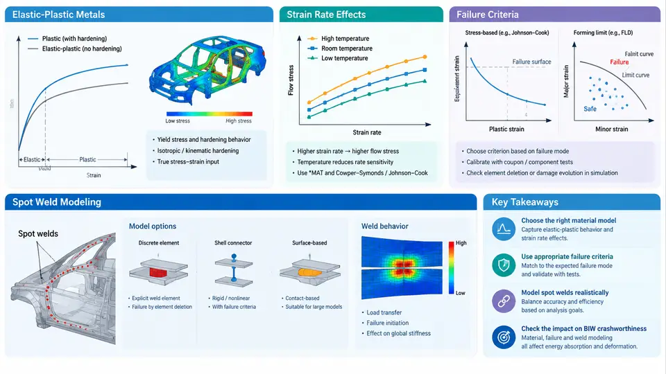
Body-in-white crashworthiness simulation is only as trustworthy as the constitutive and failure models assigned to its materials. A BIW contains mild steel, high-strength steel (HSS), advanced high-strength steel (AHSS) such as DP590/DP780, press-hardened steel (PHS) like 22MnB5, and aluminum alloys in mixed-material architectures. Each responds differently to the high strain rates and complex stress states of a crash event. This section covers the four modeling pillars that dominate prediction accuracy: elastic-plastic metal behavior, strain rate effects, failure criteria, and spot weld representation.
Elastic-Plastic Metals: MAT_PLASTIC_KINEMATIC and MAT_024
For general BIW sheet metal, LS-DYNA offers two workhorse models. *MAT_PLASTIC_KINEMATIC (MAT_003) combines isotropic and kinematic hardening through a hardening parameter β (0 = kinematic, 1 = isotropic), making it suitable when reverse loading or springback matters. *MAT_PIECEWISE_LINEAR_PLASTICITY (MAT_024) accepts a tabulated true stress–true plastic strain curve, which is the standard choice when full tensile test data are available.
The critical input is the true stress–plastic strain curve, not the engineering curve. Convert tensile data using:
ε_true = ln(1 + ε_eng)
σ_true = σ_eng · (1 + ε_eng)
ε_pl   = ε_true − σ_true / E
For DP780 with E = 210 GPa, a measured engineering ultimate of 800 MPa at 0.14 strain converts to σ_true ≈ 912 MPa at ε_pl ≈ 0.136. Feeding engineering values directly over-predicts yield and under-predicts hardening, producing energy absorption errors of 10–20% in full frontal simulations. Always extend the curve to the failure strain and define LCSS or LCSR for rate dependence.
Strain Rate Effects
BIW steels exhibit positive strain rate sensitivity: flow stress rises with loading rate. At the 1–100 s⁻¹ rates typical of crash events, DP780 may show a 15–25% flow stress increase relative to quasi-static. Two approaches are common:
- Cowper-Symonds (MAT_003): scale factor = 1 + (ε̇/C)^(1/P). Typical C = 40 s⁻¹, P = 5 for mild steel; C = 800 s⁻¹, P = 5 for DP steels. Simple but limited to a single scaling law.
- Tabulated rate curves (MAT_024 with
LCSR): define separate stress–strain curves at 0.001, 1, 10, 100, and 1000 s⁻¹ from Split Hopkinson Pressure Bar tests. LS-DYNA interpolates between curves. This is the preferred method for AHSS where rate sensitivity varies with plastic strain.
Failure Criteria
Ductile BIW metals fail by strain localization and fracture, and the strain at fracture depends strongly on stress triaxiality η = σ_m / σ_eq. Three criteria cover most BIW needs:
| Criterion | LS-DYNA Card | Best For | Key Input |
|---|---|---|---|
| Effective plastic strain | MAT_024 FAIL | Quick screening | Single ε_f |
| GISSMO | *MAT_ADD_EROSION / MAT_024 + GISSMO | AHSS, mixed stress states | ε_f vs. η curve, instability curve |
| Johnson-Cook | MAT_015 | High-rate, temperature-coupled | D1–D5 constants |
GISSMO (Generalized Incremental Stress State dependent damage model) is the current industry standard for AHSS. It tracks a damage variable D that accumulates as D = (ε_pl / ε_f(η))^n, where n is the damage exponent. Instability is triggered when D reaches 1, after which the element softens according to a defined curve until fracture. The two required curves — fracture strain vs. triaxiality and instability strain vs. triaxiality — are calibrated from a test matrix: uniaxial tension (η ≈ 0.33), plane strain (η ≈ 0.58), shear (η ≈ 0), and biaxial (η ≈ 0.67).
Calibration workflow for a DP780 coupon set:
- Run quasi-static tensile, shear, and notched tests; record force–displacement.
- Build a single-element or small mesh model per specimen with MAT_024 + GISSMO.
- Iterate ε_f(η) and instability curves until simulated force–displacement matches the test within 5% on peak and 10% on displacement to fracture.
- Validate on a component-level test (e.g., three-point bend or axial crush) before applying to full BIW.
Spot Weld Modeling
BIW assemblies contain 3,000–5,000 resistance spot welds. Modeling each as solid elements is impractical; the standard approach is a beam or solid element connecting shell mid-surfaces, with a failure criterion tied to the weld's mixed-mode capacity.
Common LS-DYNA options:
- MAT_100 (Spot Weld): beam element with resultant-based failure. Define normal and shear force/moment capacities (FN, FS, MN, MS) from coupon tests (KS-II, lap-shear, coach-peel). Failure occurs when the interaction equation (f_n/FN)² + (f_s/FS)² + (m_n/MN)² + (m_s/MS)² ≥ 1.
- MAT_240 (Beam Spot Weld): adds damage evolution and mesh-independent regularization, reducing mesh sensitivity in the heat-affected zone.
- Solid hex weld with MAT_024 + GISSMO: used when weld nugget failure mode must be captured explicitly, at higher computational cost.
Weld spacing and flange width strongly influence load transfer. A 25 mm pitch on a 16 mm flange is typical; reducing pitch to 20 mm can raise joint stiffness by 10–15% but adds mass. In optimization, weld pitch and nugget diameter are legitimate design variables, but the weld model must be calibrated first — otherwise the optimizer exploits model error rather than physical behavior.
Practical Calibration Notes
Three failure modes dominate BIW correlation errors, and each has a diagnostic signature:
- Premature element deletion in shear zones: fracture locus under-predicts ε_f at low η. Re-examine the shear coupon calibration; check that the mesh size matches the calibration gauge length.
- Delayed fracture in plane strain: instability curve set too high, allowing excessive thinning before damage triggers. Reduce ε_inst at η ≈ 0.58.
- Weld pull-out not captured: MAT_100 force capacities taken from a different nugget diameter or sheet stack. Re-derive FN/FS from the actual stack-up; weld capacity scales roughly with nugget area.
Mesh sensitivity is the silent killer. GISSMO includes a regularization option (LCSDG and ECRIT) that scales the fracture curve with element size. Without it, a 5 mm mesh and a 2 mm mesh will predict different fracture displacements for the same material. Always calibrate at the mesh size used in the full BIW model, or enable regularization and verify with a mesh convergence study on a component test.
The material model set described here — MAT_024 with tabulated rate curves, GISSMO failure, and MAT_100/MAT_240 welds — forms the baseline for the optimization studies in later chapters. Every design variable that follows (gauge, grade, weld pitch, bead layout) acts through these constitutive relationships, so calibration quality directly bounds the credibility of any subsequent optimization result.