1. Vehicle body-in-white crashworthiness op
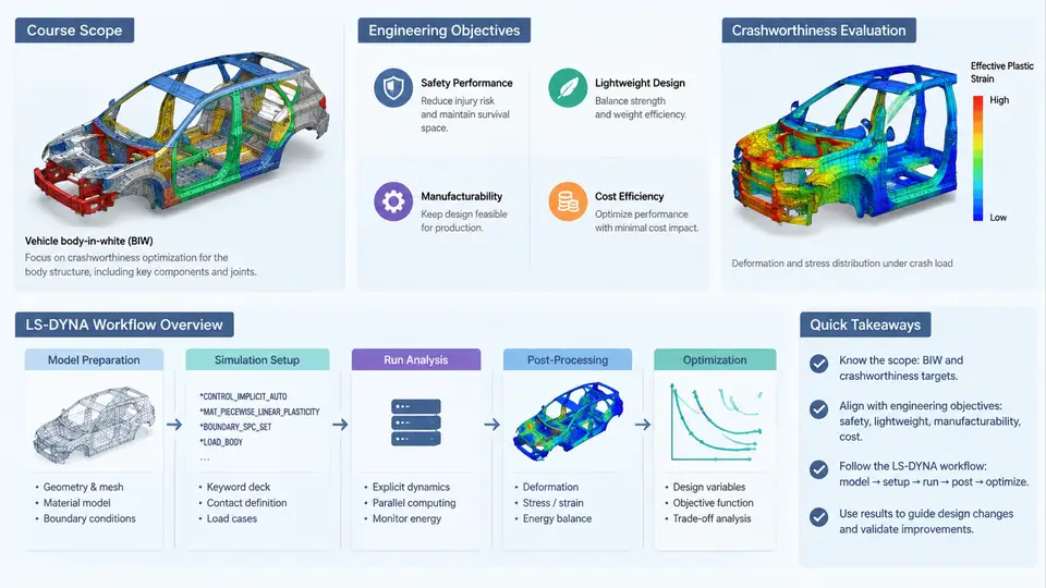
Body-in-white (BIW) crashworthiness optimization sits at the intersection of structural mechanics, explicit finite element analysis, and multidisciplinary design optimization. The BIW is the welded sheet-metal skeleton of a passenger vehicle before paint, powertrain, interior trim, and closures are installed. Although it accounts for roughly 20–30% of total vehicle mass, it governs the majority of occupant-protection performance in frontal, side, and rear impact events. This course treats the BIW as a design domain: a set of stamped panels, joints, and reinforcements whose thicknesses, grades, and topology can be tuned to meet crash targets while minimizing mass and cost.
What This Course Covers
The course spans the full engineering loop from regulatory requirements to validated, manufacturable design proposals. The major knowledge blocks are:
- Crash load cases and targets — full frontal rigid barrier (FRB), offset deformable barrier (ODB), side pole and MDB, rear impact, and roof crush, each with its own injury criteria and structural acceptance thresholds.
- LS-DYNA model construction — shell element meshing, material cards for mild, high-strength, and ultra-high-strength steels, spot-weld and adhesive connection modeling, and contact definitions.
- Solution control — explicit time integration, mass scaling, hourglass control, and termination criteria.
- Design of experiments and surrogate modeling — parameter screening, response surface or Kriging metamodels, and multi-objective optimization algorithms.
- Robustness and manufacturability — accounting for thickness tolerances, material scatter, and stamping feasibility in the optimized result.
The scope deliberately excludes detailed occupant restraint system design and full vehicle NVH, except where they impose constraints on the BIW structure.
Engineering Objectives
Crashworthiness optimization of a BIW is never a single-objective problem. The engineer must simultaneously satisfy several competing requirements:
| Objective | Typical Metric | Direction |
|---|---|---|
| Occupant safety | B-pillar intrusion, chest deceleration, femur load | Minimize |
| Structural integrity | Frontal crush stroke, cabin survival space | Maximize / maintain |
| Mass efficiency | BIW mass, mass per unit energy absorbed | Minimize |
| Manufacturing cost | Number of dies, material grade cost, weld count | Minimize |
| Modal performance | First torsional and bending frequencies | Maximize / constrain |
A practical optimization problem is therefore formulated as a constrained multi-objective problem. For example, minimize BIW mass subject to: B-pillar intrusion ≤ 120 mm in side MDB, front bumper maximum intrusion ≤ 400 mm in FRB, and first torsional frequency ≥ 35 Hz. The design variables are typically panel thicknesses (continuous, 0.6–2.5 mm), material grades (discrete), and sometimes bead or rib layout parameters.
Engineering note: In real projects, the crash pulse and occupant response are coupled. A stiffer front end reduces intrusion but raises deceleration. The optimizer must therefore work with a surrogate that captures this trade-off, not just a single scalar objective.
The LS-DYNA Workflow Overview
LS-DYNA is an explicit finite element solver widely used for crash simulation because it handles large deformation, contact, and material failure efficiently. The BIW optimization workflow using LS-DYNA follows a structured sequence:
- Geometry preparation and meshing — Import CAD surfaces, midsurface the sheet metal, and mesh with Belytschko-Tsay shell elements. Target element size is typically 5–8 mm in crash-critical zones and 10–15 mm elsewhere. Check for warpage, aspect ratio, and Jacobian errors.
- Material and property assignment — Assign
*MAT_PIECEWISE_LINEAR_PLASTICITYor*MAT_024for mild steel,*MAT_037for high-strength steel, and*MAT_ADD_EROSIONwhere failure is expected. Define thickness per part. - Connection modeling — Represent spot welds with
*CONSTRAINED_SPOTWELDor solid elements; use*CONTACT_AUTOMATIC_SINGLE_SURFACEfor self-contact and*CONTACT_AUTOMATIC_SURFACE_TO_SURFACEfor barrier interaction. - Boundary and initial conditions — Apply initial velocity (e.g., 50 km/h for FRB), define rigid walls, and set termination time based on event duration (typically 80–120 ms).
- Solution and mass scaling — Use
*CONTROL_TIMESTEPwith a target time step. Apply mass scaling only to stable, non-critical regions to avoid artificial inertia effects. - Post-processing — Extract intrusion, acceleration, and energy curves using LS-PrePost or a Python script. Verify energy balance: hourglass energy should remain below 5% of total energy.
- Design iteration — Feed results into the optimizer (e.g., LS-OPT, modeFRONTIER, or a custom Python loop). Update thicknesses or grades, re-mesh if needed, and re-run.
The following SVG illustrates the data and decision flow across one optimization cycle, from parameter definition to convergence check.
Practical Considerations and Common Pitfalls
New analysts often treat the LS-DYNA run as the center of the workflow. In practice, the quality of the optimization depends more on the surrogate model and the design space definition. A few concrete guidelines:
- Start with a screening DOE. Use a fractional factorial or Plackett-Burman design with 8–16 runs to identify the 5–8 most influential thickness variables. Running a full optimization on 30 variables is computationally wasteful.
- Check energy balance before trusting results. If hourglass energy exceeds 5% of internal energy, refine the mesh or switch to a fully integrated shell formulation. If added mass from mass scaling exceeds 3% of total mass, reduce the scaling factor.
- Constrain the design space to manufacturable limits. A thickness of 0.3 mm is not producible; a grade change may require different weld schedules. The optimizer will exploit unconstrained regions if you let it.
- Validate the surrogate. After optimization, run the predicted optimum through LS-DYNA. A surrogate error above 5% on intrusion or acceleration means the metamodel needs more samples or a different kernel.
Warning: Do not use mass scaling on the front crash rails or B-pillar. These regions undergo large plastic deformation and their stable time step is already small. Scaling mass there introduces artificial inertia that will under-predict intrusion and over-predict deceleration.
What a Successful Outcome Looks Like
At the end of a BIW crashworthiness optimization study, the deliverable is not a single number. It is a Pareto front: a set of non-dominated designs showing the trade-off between mass and intrusion, or between mass and deceleration. The engineer selects one design based on program priorities, then verifies it with a full LS-DYNA run and a manufacturability review. Typical acceptance criteria for a frontal load case are: maximum firewall intrusion ≤ 150 mm, peak B-pillar acceleration ≤ 40 g, and no weld separation in the primary load path. For side impact, B-pillar intrusion at occupant hip height ≤ 120 mm and door trim velocity ≤ 8 m/s are common targets.
The next chapters will build each of these elements in detail, starting with the crash load cases and their regulatory and consumer-test definitions.