4. Material models for forming history
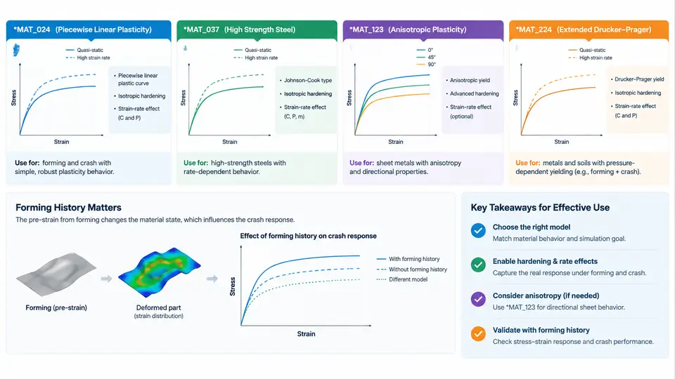
When a stamped or hydroformed part is transferred into a crash model, the material card must reproduce the state the blank actually reached during forming: accumulated plastic strain, altered yield surface, thickness reduction, and—for advanced steels—transformation-induced phase fractions. LS-DYNA offers several elastoplastic material models that can carry this history. The four most common in body-in-white crash work are *MAT_024 (PIECEWISE_LINEAR_PLASTICITY), *MAT_037 (TRANSVERSELY_ANISOTROPIC_ELASTIC_PLASTIC), *MAT_123 (MODIFIED_PIECEWISE_LINEAR_PLASTICITY), and *MAT_224 (TABULATED_JOHNSON_COOK). They differ in how yield stress is defined, how anisotropy is treated, how strain rate is interpolated, and whether damage or phase transformation can be tracked. Choosing the wrong one, or mapping the wrong history variables into it, is one of the most frequent sources of non-physical crash results.
4.1 What "Forming History" Actually Means in the Material Card
Forming history enters a crash model through three channels. First, the initial plastic strain EPS (or the effective plastic strain field written by the forming solver) shifts the starting point on the hardening curve, so the material is already work-hardened before impact. Second, the thickness field modifies the section's bending and membrane stiffness. Third, for anisotropic or phase-transforming grades, the texture or phase state changes the yield locus and the rate sensitivity. A material model is therefore only "history-capable" if it exposes these variables as initial conditions and reads them consistently during the crash step.
EPS will land on the wrong stress level and the part will appear artificially soft or stiff.
4.2 *MAT_024 — PIECEWISE_LINEAR_PLASTICITY
*MAT_024 is the workhorse isotropic von Mises model. Yield stress is defined either by a tabulated curve (LCSS) or by the bilinear pair SIGY and ETAN. Strain-rate sensitivity is optional and is supplied through LCSR, a set of scaled yield curves indexed by effective plastic strain rate. The card also accepts an initial effective plastic strain EPS per integration point, which is exactly the field written by a forming solver.
Typical input for a mild steel after forming:
*MAT_PIECEWISE_LINEAR_PLASTICITY
$#   mid        ro         e        pr      sigy      etan      fail       tdel
         1  7.85e-9  210000.0       0.3       0.0       0.0       0.0       0.0
$#    lcss      lcsr        vp
         100       200       0.0
$#    eps       es
       0.0       0.0
Here LCSS = 100 is the true-stress vs. plastic-strain curve, LCSR = 200 is the rate-scaling table, and EPS is left at zero because the mapped history is applied through *INITIAL_STRESS_SHELL or the *INITIAL_STRESS_SOLID path. The model is cheap, robust, and adequate for mild steels and many aluminum alloys where anisotropy is weak. Its limitation is that it cannot represent directional yield or the Bauschinger effect, so springback-driven residual stress patterns are only approximated.
4.3 *MAT_037 — TRANSVERSELY_ANISOTROPIC_ELASTIC_PLASTIC
*MAT_037 extends the isotropic framework with a Hill-type quadratic yield function. The card takes three Lankford coefficients R, R45, and R90 (or the full anisotropic matrix), plus the same LCSS/LCSR hardening and rate inputs as *MAT_024. It is the natural choice for cold-rolled sheet where the rolling direction produces measurable differences in yield and thinning behavior.
For a DC04-grade sheet with R0 = 1.8, R45 = 1.4, R90 = 2.1, the yield locus is elongated along the transverse direction. After forming, the mapped EPS field is no longer a scalar indicator of "how hard" the material is—it interacts with the local stress triaxiality through the anisotropic coefficients. In practice this means the crash card must retain the same R values used in the forming run; changing them silently redefines the yield surface and invalidates the history mapping.
4.4 *MAT_123 — MODIFIED_PIECEWISE_LINEAR_PLASTICITY
*MAT_123 is a modified version of *MAT_024 that adds an optional damage/erosion flag and a more flexible rate formulation. The hardening curve is still tabulated, but the card exposes LCSS, LCSR, and a failure strain FAIL that can be used to delete elements once the effective plastic strain exceeds a threshold. This makes it attractive for crash models where the formed part is expected to tear.
The practical difference from *MAT_024 is the treatment of the rate term. *MAT_123 allows the rate scaling to be applied to the entire curve rather than to a single reference stress, which improves accuracy for steels that show pronounced rate sensitivity at high strain rates (102–104 s-1). The trade-off is a slightly higher computational cost and a more careful calibration of LCSR.
4.5 *MAT_224 — TABULATED_JOHNSON_COOK
*MAT_224 is the most general of the four. Instead of a single hardening curve, it accepts a table of flow stress as a function of effective plastic strain, strain rate, and temperature. The card is defined by LCSS (a 3D table), LCSR, and optional thermal softening data. It also supports an initial plastic strain field and a damage initiation table, which makes it suitable for press-hardened steels (PHS) and other grades where the forming step involves both hardening and phase transformation.
For a 22MnB5 PHS after hot stamping, the crash card typically uses *MAT_224 with a flow-stress table covering 0.001–5000 s-1 and a martensitic phase fraction mapped from the forming solver. The initial EPS field is small (the material is already fully martensitic), but the rate table is essential because the crash response is dominated by rate sensitivity rather than by prior work hardening.
4.6 Hardening and Strain-Rate Effects: What to Calibrate
All four models share the same conceptual hardening input: a true-stress vs. effective-plastic-strain curve. The curve should be obtained from a tensile test up to necking and extrapolated beyond necking using a Swift or Voce fit. For crash work, the extrapolation matters because the forming step may push the material to 0.3–0.5 effective plastic strain, well beyond the uniform elongation of a standard tensile specimen.
Strain-rate effects are handled differently. *MAT_024 and *MAT_037 use LCSR as a set of scale factors applied to the quasi-static curve. *MAT_123 allows the rate scaling to be applied more flexibly. *MAT_224 uses a full 3D table, which is the only option that can capture the interaction between rate and temperature for PHS. A practical calibration sequence is:
- Fit the quasi-static hardening curve from tensile data (true stress, true plastic strain).
- Run Split-Hopkinson pressure bar (SHPB) tests at 500, 1000, and 2000 s-1 to obtain rate-scaled curves.
- Build
LCSRas the ratio of dynamic to quasi-static flow stress at a reference plastic strain (typically 0.05–0.10). - For
*MAT_224, assemble the 3D table directly from the SHPB data and add thermal softening from elevated-temperature tests if the forming step was hot.
EPS and compare the resulting flow stress against the forming solver's final stress. A mismatch greater than 5% usually indicates a curve or unit inconsistency.
4.7 Common Failure Modes and Troubleshooting
| Symptom | Likely cause | Corrective action |
|---|---|---|
| Part appears too soft in crash | EPS not mapped or mapped as zero |
Verify *INITIAL_STRESS_SHELL / *INITIAL_STRESS_SOLID reads the forming result file |
| Yield stress too high at low strain | Hardening curve in crash card differs from forming card | Use the identical LCSS curve in both decks |
| Unrealistic thinning in crash | Thickness field not transferred | Map shell thickness from the forming result; check *ELEMENT_SHELL_THICKNESS |
| Rate sensitivity ignored | LCSR missing or set to zero |
Add rate table; confirm units of strain rate (s-1) |
| Anisotropy lost after mapping | R values changed between forming and crash |
Keep R0, R45, R90 identical in both decks |
4.8 Summary
The choice among *MAT_024, *MAT_037, *MAT_123, and *MAT_224 is driven by what the forming history actually changed. If only the plastic strain level matters, *MAT_024 is sufficient and cheapest. If the sheet has directional yield, *MAT_037 preserves the yield locus. If the formed part is expected to tear, *MAT_123 adds erosion. If the grade is rate-sensitive or phase-transforming, *MAT_224 is the only model that carries the full table. In every case, the hardening curve, rate table, and anisotropy parameters must be identical between the forming and crash decks; the mapped history variables are only meaningful if the constitutive surface they are applied to is the same one that generated them.