1. High-fidelity contact and impact modelin
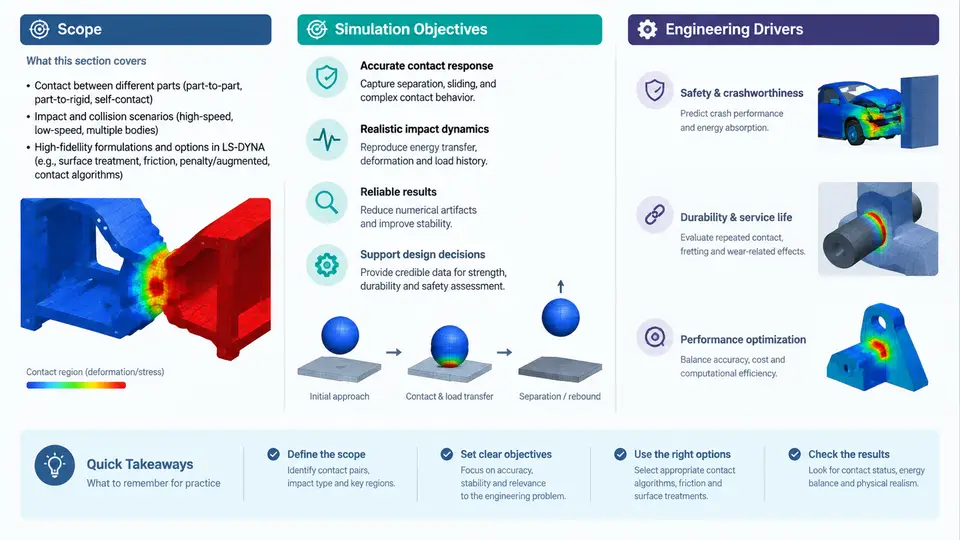
Impact simulation is one of the few analysis domains where the physics of interest is concentrated into milliseconds, yet the engineering consequences persist for the entire product lifecycle. A vehicle frontal crash, a drop-tested consumer device, a bird strike on a fan blade, or a ballistic penetration event all share the same computational signature: large deformations, moving material interfaces, strain rates spanning several decades, and energy transfer that must be conserved to within a few percent. LS-DYNA was built for exactly this class of problem, and its contact algorithms are the component that most often determines whether a simulation is predictive or merely decorative.
This chapter establishes the scope of high-fidelity contact and impact modeling, defines what "high fidelity" means in measurable terms, and explains the engineering drivers that justify the additional modeling effort. Subsequent chapters will treat penalty formulations, contact stiffness, friction, tiebreak, erosion, and adaptive remeshing in detail; here we build the conceptual and quantitative foundation those chapters depend on.
What "High Fidelity" Actually Means
Fidelity in impact simulation is not a single metric. It is a composite of four properties that must hold simultaneously:
- Kinematic accuracy — predicted displacements, rotations, and deformation modes match physical observation within an agreed tolerance, typically 5–10% on peak intrusion or deflection.
- Energy consistency — the global energy balance (internal + kinetic + contact + hourglass + damping) closes to within 1–2% of initial kinetic energy, with no unexplained growth in hourglass or contact energy.
- Contact robustness — no spurious penetration beyond a defined threshold, no contact force oscillations that are numerical rather than physical, and stable behavior under mesh refinement.
- Convergence under refinement — results change monotonically and boundedly as element size decreases, rather than diverging or oscillating.
A model that satisfies kinematic accuracy but violates energy consistency is not high fidelity; it is a coincidence. This distinction matters because impact simulations are frequently used to make safety-critical decisions, and a plausible-looking animation can mask a fundamentally broken contact definition.
The Engineering Drivers
Four drivers push practitioners toward high-fidelity contact modeling rather than simplified approaches:
Regulatory and certification requirements. FMVSS 208, Euro NCAP, and similar regimes specify occupant injury criteria (HIC, chest deflection, femur load) that depend directly on structural intrusion, which in turn depends on contact force distribution. A 10% error in contact stiffness can shift HIC by 50 points or more near a threshold.
Design space exploration. When a team evaluates dozens of gauge, material, and topology variants, the ranking of designs must be reliable. Simplified contact models often preserve the ranking of grossly different designs but fail to discriminate between closely competing ones — precisely the regime where optimization value is highest.
Failure mode prediction. Spot weld rupture, adhesive debonding, and material erosion are contact-driven failure modes. Predicting whether a joint survives requires tiebreak or cohesive contact with calibrated normal and shear strengths, not a tied constraint that never releases.
Cost of physical testing. A full-scale crash test costs tens of thousands of dollars and weeks of lead time. A drop test or sled test is cheaper but still consumes schedule. High-fidelity simulation substitutes for a meaningful fraction of these tests only if it has been validated against them.
Scope of the Modeling Domain
The scope of contact and impact modeling in LS-DYNA spans several physical regimes that require different algorithmic treatment:
| Regime | Typical strain rate | Dominant contact behavior | Primary LS-DYNA keywords |
|---|---|---|---|
| Quasi-static crush | 10⁻³ – 10⁰ s⁻¹ | Stable, large sliding contact | *CONTACT_AUTOMATIC_SINGLE_SURFACE |
| Low-speed impact | 10⁰ – 10² s⁻¹ | Elastic-plastic contact, rebound | *CONTACT_AUTOMATIC_SURFACE_TO_SURFACE |
| High-speed impact | 10² – 10⁴ s⁻¹ | Erosion, adiabatic heating, phase change | *CONTACT_ERODING_SURFACE_TO_SURFACE |
| Penetration / ballistic | 10⁴ – 10⁶ s⁻¹ | Material failure, debris contact | *CONTACT_ERODING_NODES_TO_SURFACE |
Each regime imposes different requirements on time step, element formulation, and contact stiffness. A model calibrated for quasi-static crush will not automatically perform well at ballistic velocities, because the dominant energy dissipation mechanisms change.
Simulation Objectives and Their Measurable Outcomes
Before building any model, the analyst should state the objective in terms that can be verified. Three common objective types and their verification criteria:
- Peak force prediction. Objective: predict maximum contact force within 10%. Verification: compare force-time history against a drop tower or servo-hydraulic test; check that the peak occurs at the correct time and that the unloading slope is physical.
- Intrusion prediction. Objective: predict maximum intrusion at specified measurement points within 5 mm. Verification: compare against a physical test with displacement transducers; check that the deformation mode (bending vs. folding) matches.
- Failure initiation prediction. Objective: predict whether a joint or panel fails. Verification: compare against tests that bracket the failure threshold; check that the predicted failure location matches the observed crack or rupture path.
These objectives are not interchangeable. A model tuned for peak force may over-predict intrusion if the contact stiffness is artificially high. The analyst must decide which objective dominates and accept the corresponding trade-offs.
Energy Balance as the Primary Diagnostic
The single most useful diagnostic in an impact simulation is the energy balance. LS-DYNA reports global energies in the glstat file and contact energies in the matsum and sleep files. The governing relation is:
E_total = E_kinetic + E_internal + E_contact + E_hourglass + E_damping + E_sliding

For a well-posed model:
  |E_total - E_total(0)| / E_kinetic(0) < 0.02
  E_hourglass / E_internal < 0.05
  E_contact should be positive and bounded
If hourglass energy exceeds 5% of internal energy, the element formulation or mesh is inadequate. If contact energy grows without bound, the contact stiffness or penalty scale factor is too high. If total energy drifts by more than 2%, there is likely a numerical instability or an unphysical energy source.
glstat before interpreting any result. A model with 15% hourglass energy may show the "right" crush shape for the wrong reason.
Workflow Overview
The figure below maps the relationship between the engineering decision, the modeling choices it drives, and the verification loop that closes the process. It is not a linear procedure; the verification step frequently sends the analyst back to contact definition or mesh refinement.
Practical Starting Point: A Minimal Reproducible Example
To make the scope concrete, consider a simple but representative case: a 2 kg rigid impactor striking a 1.5 mm thick DP600 steel plate at 7 m/s. The objective is to predict peak contact force within 10% of a drop tower measurement.
Key inputs for this example (illustrative values, not measured data):
- Plate: 200 mm × 200 mm, shell elements, Belytschko-Tsay formulation, 2 mm characteristic length
- Material: *MAT_PIECEWISE_LINEAR_PLASTICITY with DP600 hardening curve, strain rate via *DEFINE_CURVE
- Impactor: rigid hemisphere, R = 25 mm, mass 5 kg
- Contact: *CONTACT_AUTOMATIC_SURFACE_TO_SURFACE, SOFT = 1, friction 0.15
- Termination: 15 ms, mass scaling limited to 2% added mass
Expected observable behavior: the force-time history should show an initial elastic rise, a peak near 1.5–2.5 ms, and a gradual unloading as the plate absorbs energy through plastic hinge formation. If the contact energy exceeds 10% of internal energy, the penalty stiffness is too high; if hourglass energy exceeds 5%, the shell formulation or mesh density needs revision. If the peak force is more than 15% above the test value, check whether the contact thickness offset is correctly defined for the shell mid-surface.
This example illustrates the full loop: a decision (does the plate survive?), an objective (peak force within 10%), modeling choices, diagnostics, and verification. Every subsequent chapter in this course elaborates one part of this loop.
Summary
High-fidelity contact and impact modeling in LS-DYNA is defined by four measurable properties — kinematic accuracy, energy consistency, contact robustness, and convergence under refinement — and is driven by regulatory, design-exploration, failure-prediction, and cost considerations. The scope spans quasi-static crush through ballistic penetration, each regime requiring different contact algorithms and element treatments. The energy balance reported in glstat is the primary diagnostic, and the workflow is inherently iterative: verification against test data or convergence criteria determines whether the model is fit for the decision it is meant to support.