4. Material modeling for crashworthiness
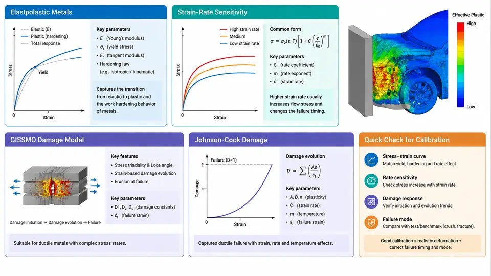
In a frontal impact simulation, the accuracy of the predicted deformation pattern, intrusion, and occupant loading depends far more on the constitutive and failure models than on mesh density or contact settings. A body-in-white (BIW) rail that folds correctly in the physical test but tears prematurely in the model usually points to a failure model that was never calibrated for the actual stress state and strain rate. This chapter covers the material modeling chain used in production crashworthiness work: elastoplasticity for the hardening response, strain-rate sensitivity for high-speed loading, and damage/failure models — GISSMO and Johnson-Cook — together with the calibration workflow that ties them to coupon test data.
Elastoplastic Metals: Hardening and the True Stress–Strain Curve
Crash-relevant metals (HSLA steels, DP590/DP780, 6xxx aluminum, press-hardened boron steel) are modeled with an elastoplastic formulation: linear elastic up to yield, then plastic flow with isotropic hardening. LS-DYNA's *MAT_PIECEWISE_LINEAR_PLASTICITY (*MAT_024) is the workhorse for this. The critical practical point is that the input curve must be true stress vs. plastic strain, not engineering stress–strain. Convert the tensile test data using:
sigma_true = sigma_eng * (1 + eps_eng)
eps_true   = ln(1 + eps_eng)
eps_pl     = eps_true - sigma_true / E
For a DP780 coupon with E = 210 GPa, yield at 480 MPa engineering, and UTS of 820 MPa at 14% engineering strain, the true UTS is approximately 820 × 1.14 = 935 MPa at a true strain of ln(1.14) = 0.131, giving a plastic strain of about 0.127. Feeding engineering data directly into *MAT_024 underestimates the flow stress at large strain by 10–15% and produces rails that are too soft. Beyond necking, the curve must be extrapolated — a power-law or linear extension to the failure strain is standard, and the extrapolation choice should be documented because it directly affects energy absorption.
Strain-Rate Sensitivity
Frontal impact strains develop at 10²–10³ s⁻¹, where BCC steels show a pronounced yield-strength increase (commonly 30–60% at 1000 s⁻¹ for mild and HSLA grades), while FCC aluminum is far less sensitive. LS-DYNA offers two practical routes:
- Rate-dependent plasticity via
*MAT_024withLCSS: supply a table of scale factors on the flow curve versus effective plastic strain rate. This is the most common approach for steels. - Cowper–Symonds / Johnson-Cook rate terms: a multiplicative factor on yield, e.g.
1 + C·ln(ε̇/ε̇₀)in Johnson-Cook, or1 + (ε̇/D)^(1/p)in Cowper–Symonds.
Calibration requires split-Hopkinson pressure bar (SHPB) data at several rates (e.g. 0.001, 1, 100, 1000 s⁻¹). A common pitfall is applying a single rate factor uniformly across all plastic strains; in reality the rate sensitivity often decreases at large strain, so the scale-factor table should be built per plastic strain level if the data supports it.
Damage and Failure: GISSMO vs. Johnson-Cook
Ductile fracture in crash is stress-state dependent. The triaxiality η = σ_m / σ_vm controls void growth: shear-dominated states (η ≈ 0) and biaxial states (η ≈ 0.6–0.7) fail at very different equivalent plastic strains. Two models dominate:
| Model | Formulation | Best suited for | Key inputs |
|---|---|---|---|
| Johnson-Cook damage | ε_f = (D1 + D2·exp(D3·η))·(1 + D4·ln ε̇*)·(1 + D5·T*) | High-rate, thermal-coupled problems; aerospace and some aluminum crash | D1–D5, rate and temperature terms |
| GISSMO | Damage accumulation D = (ε_p/ε_f(η))^n, with instability and regularization | Sheet-metal BIW steels, shell models, mesh-size-sensitive fracture | ε_f vs. η curve, n, instability curve, regularization exponent |
GISSMO (*MAT_ADD_EROSION with GISSMO or the dedicated keyword) is preferred for body structures because it separates damage from instability, allowing the model to capture the diffuse necking that precedes fracture — essential for predicting fold initiation in rails. Johnson-Cook damage is simpler but tends to over-predict failure under shear and does not handle mesh regularization natively.
Failure Calibration Workflow
Calibration is a coupon-driven process. The standard specimen set covers the triaxiality range:
- Uniaxial tension (η ≈ 0.33) — establishes the hardening curve and baseline ε_f.
- Notched tension (R = 2, 5, 10 mm; η ≈ 0.4–0.55) — intermediate triaxiality.
- Central hole / plane strain (η ≈ 0.6) — biaxial-dominant.
- Shear specimen (η ≈ 0–0.1) — critical for shear fracture in bending-dominated regions.
- Butterfly / biaxial (η up to 0.7) — completes the curve.
Each specimen is simulated with a fine, regular mesh (0.5–1.0 mm solid or shell with element size matching the intended BIW mesh). The failure strain is extracted by matching the simulated force–displacement curve to the test: the point where the simulated curve drops is tuned by adjusting ε_f at that η. The resulting ε_f(η) curve is then fitted and entered into GISSMO. The regularization exponent n is calibrated by running the same specimen at two or three mesh sizes (e.g. 0.5, 1.0, 2.0 mm) and adjusting n until the fracture displacement is mesh-insensitive.
Verification and Result Interpretation
After calibration, verify on a component-level test — a three-point bend or axial crush of a closed-hat section — before applying to the full BIW. Compare the force–displacement curve, the peak load, the mean crush force, and the final deformation mode. A well-calibrated GISSMO model should reproduce the peak within 5–10% and the mean crush force within 5%. If the model is too stiff, revisit the rate-dependent scale factors; if it fractures too early, revisit the shear branch of the failure curve. Only after component verification should the material card be released for full-vehicle frontal impact runs.
The figure summarizes the full chain: hardening and rate data feed the constitutive model, the coupon set defines the failure locus, and mesh regularization ensures the calibrated ε_f(η) transfers across element sizes. Treating these as one integrated calibration — rather than four independent keyword entries — is what separates a model that predicts folding from one that predicts tearing.