1. Crash model quality framework
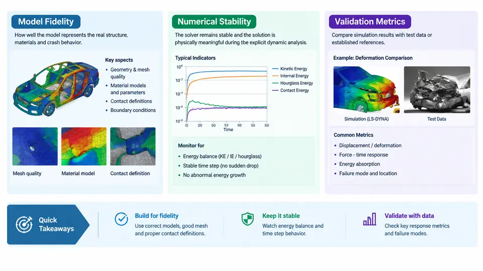
In LS-DYNA explicit crash simulation, "the model runs" is not the same as "the model is trustworthy." A model can terminate normally with zero error messages and still produce a physically meaningless result — a vehicle that absorbs 40% too much energy, a dummy chest deflection that never exceeds 20 mm, or hourglass energy that quietly consumes a third of the internal energy budget. The purpose of a crash model quality framework is to make the difference between running and being right explicit, measurable, and auditable.
This chapter defines the three pillars of that framework — model fidelity, numerical stability, and validation metrics — and shows how they interact inside a standard LS-DYNA explicit dynamics workflow. The goal is not to introduce a checklist to be filled in mechanically, but to establish the vocabulary and the causal reasoning that every later chapter will build on.
Model Fidelity: What the Model Represents
Model fidelity is the degree to which the discretized model reproduces the physical behavior of the real structure under the intended load case. It is a property of the modeling decisions, not of the solver run. Fidelity is degraded by geometry simplification, mesh coarseness, material model mismatch, missing joints, and incorrect boundary conditions — and these degradations are largely independent of whether the simulation converges.
In practice, fidelity is assessed along several axes:
- Geometric fidelity — whether structural details that carry load (spot weld flanges, crush initiators, gussets, hinge reinforcements) are represented. A B-pillar modeled as a smooth shell without its bead pattern will under-predict folding resistance.
- Material fidelity — whether the constitutive model and its parameters capture the relevant strain-rate, failure, and hardening behavior. Using
*MAT_PIECEWISE_LINEAR_PLASTICITYfor a press-hardened steel that actually fails by brittle cracking is a fidelity error, not a stability error. - Connection fidelity — whether spot welds, adhesive bonds, bolts, and seams transfer load with realistic stiffness and failure. A welded joint modeled as rigid will not release at the correct force.
- Boundary and loading fidelity — whether the barrier, sled, or impactor is represented with correct mass, velocity, and contact stiffness.
A useful working definition: fidelity is the set of modeling assumptions that remain valid after the simulation ends. If the model's assumptions break down during the event — for example, a shell element that should fail in tension instead stretches indefinitely — the result is not a stability failure but a fidelity failure that may masquerade as one.
Numerical Stability: Whether the Solution Remains Physical
Numerical stability in explicit dynamics means the time integration remains bounded and the discrete solution does not diverge from the physical solution due to numerical artifacts. LS-DYNA's central difference scheme is conditionally stable: the critical time step is governed by the smallest element and the highest wave speed,
Δt_crit = L_min / c, c = sqrt(E / ρ)where L_min is the characteristic element length and c is the acoustic wave speed. When the time step exceeds Δt_crit, the solution grows without bound. In practice, instability rarely appears as a clean divergence; it appears as:
- Negative volume errors in solid elements or inverted shell elements
- Explosive growth of hourglass energy relative to internal energy
- Contact penetration that grows monotonically instead of oscillating around a small value
- Element erosion cascades that remove load-carrying structure prematurely
- Mass scaling that inflates the model's kinetic energy beyond acceptable limits
The critical distinction is that stability is necessary but not sufficient for fidelity. A model can be perfectly stable and completely wrong. Conversely, a fidelity-correct model can be numerically unstable if the time step, contact stiffness, or hourglass control is poorly chosen. The framework must therefore treat them as separate diagnostic axes.
Validation Metrics: How We Know the Model Is Right
Validation metrics quantify the agreement between simulation output and physical reference data — typically sled test or full-scale crash test measurements. In LS-DYNA workflows, the most common metrics are applied to time-history channels: acceleration, velocity, displacement, force, and energy.
Three metric families are widely used:
| Metric | What it measures | Typical acceptance |
|---|---|---|
| Peak error | Difference in maximum value of a channel | < 10–15% for acceleration peaks |
| Time-of-peak error | Phase shift between simulated and test peaks | < 5–10 ms |
| CORrelation (CORA / ISO 18571) | Combined magnitude, phase, and shape agreement | > 0.7 acceptable, > 0.85 good |
Energy balance is a special validation metric because it is internal to the simulation and requires no test data. The total energy at any time should satisfy:
E_total = E_kinetic + E_internal + E_hourglass + E_sliding + E_damping + E_externalFor a well-behaved crash model, hourglass energy should remain below roughly 5% of peak internal energy, and the energy balance error (initial total minus current total) should stay below 1–2%. These thresholds are not arbitrary: they reflect the point at which numerical dissipation begins to compete with physical energy absorption.
How the Three Pillars Interact
The framework is not a checklist of independent items. The three pillars form a diagnostic loop, and the SVG below shows how a single symptom — say, a 30% under-prediction of intrusion — is traced back to its root cause through the framework.
The loop works as follows. A validation metric flags a discrepancy. The engineer then asks two questions in sequence: first, is the energy balance acceptable? If hourglass energy or mass scaling has corrupted the solution, the discrepancy is a stability artifact and must be fixed before any fidelity conclusion can be drawn. Second, does the deformation mode match the physical test? If the folding pattern, failure location, or joint release sequence differs, the discrepancy is a fidelity issue. Only when both checks pass does the remaining error represent a genuine modeling gap that requires parameter calibration or test-data review.
Applying the Framework: A Worked Example
Consider a frontal offset crash model of a body-in-white with a 40% overlap deformable barrier at 64 km/h. The simulation terminates normally at 120 ms. The B-pillar intrusion at the door latch is 85 mm; the sled test measured 120 mm. The engineer must decide whether this is a stability problem, a fidelity problem, or both.
Step 1 — Energy audit. Extract the energy summary from glstat and matsum. Suppose the peak internal energy is 48 kJ, and hourglass energy peaks at 4.2 kJ — about 8.8% of internal energy. This exceeds the 5% guideline. The hourglass control is under-damped for the coarse mesh in the B-pillar. This is a stability-side contributor: numerical energy is being absorbed by hourglass modes instead of by physical deformation, which artificially stiffens the structure and reduces intrusion.
Step 2 — Deformation mode check. Compare the simulated B-pillar folding pattern with the high-speed video. If the simulation shows a single large fold where the test shows two smaller folds, the mesh is too coarse to resolve the fold wavelength. This is a fidelity-side contributor.
Step 3 — Corrective action. Refine the B-pillar mesh from 8 mm to 5 mm characteristic length, switch from *HOURGLASS type 1 (standard) to type 4 (Flanagan-Belytschko stiffness form) with a coefficient of 0.05, and re-run. After the re-run, hourglass energy drops to 1.8% of internal energy, and intrusion increases to 112 mm. The remaining 8 mm gap is now a genuine fidelity question — likely spot weld failure timing or material strain-rate sensitivity — and can be addressed with test-correlated calibration.
Framework Summary
The three pillars are not sequential steps but simultaneous constraints. A model is qualified only when all three are satisfied:
- Fidelity — the model's assumptions remain valid throughout the event, verified by deformation mode and failure sequence comparison.
- Stability — the time step, hourglass control, contact stiffness, and mass scaling keep the solution bounded and the energy balance closed.
- Validation — quantitative metrics (peak, phase, CORA, energy balance) confirm agreement with physical reference data within defined tolerances.
Every subsequent chapter in this course addresses one or more of these pillars in depth: mesh quality and time-step control, hourglass and contact stability, material and failure modeling fidelity, and the statistical treatment of validation metrics. The framework introduced here is the lens through which all of that material should be read.