4. Experimental characterization for failur
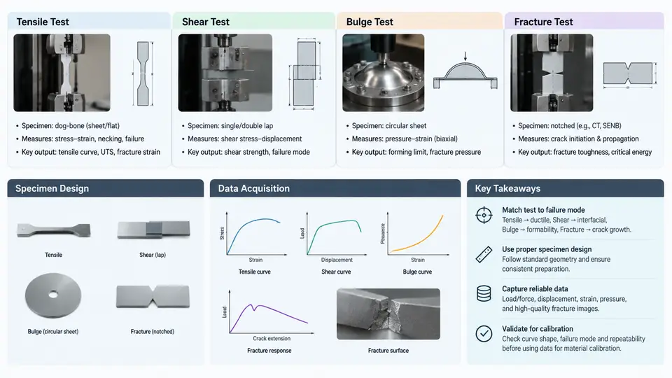
Failure calibration in LS-DYNA is only as trustworthy as the experimental data that feeds it. A material card such as *MAT_024 with *MAT_ADD_EROSION, or a ductile damage model like *MAT_224 (GISSMO) or *MAT_ADD_DAMAGE_GISSMO, requires a failure locus — the equivalent plastic strain at fracture as a function of stress triaxiality and, for many sheet metals, the Lode angle parameter. No single coupon geometry can populate that locus. The calibration engineer must therefore assemble a test matrix that spans stress states from near-uniaxial compression through shear, uniaxial tension, plane-strain tension, and biaxial tension. This section covers the four canonical test families — tensile, shear, bulge, and fracture — together with specimen design and the data-acquisition chain that converts raw signals into usable input curves.
Stress-State Coverage and the Triaxiality Map
Stress triaxiality is defined as η = σm/σeq, the ratio of mean (hydrostatic) stress to von Mises equivalent stress. Shear-dominated specimens sit near η ≈ 0, notched round bars and plane-strain specimens occupy η ≈ 0.33–0.6, and bulge or biaxial specimens reach η ≈ 0.66–0.75. Because ductile metals lose ductility rapidly as triaxiality rises, the failure locus is steeply sloped, and gaps in the test matrix translate directly into interpolation error in the calibrated model. A practical target is at least five distinct stress states, with two or more replicates each to quantify scatter.
Tensile Tests: Smooth and Notched Round Bars
The smooth round-bar tensile test establishes the hardening curve up to necking, but its post-necking behavior is not directly measurable from crosshead displacement. For failure calibration, notched round bars are more valuable: the notch radius controls triaxiality, with R = 20 mm giving η ≈ 0.25, R = 10 mm giving η ≈ 0.33, and R = 4 mm pushing η above 0.45. Specimens are typically machined to ASTM E8 proportions with a gauge diameter of 6 mm and a notch root diameter of 3–4 mm.
Acquisition uses a clip-on or laser extensometer across the notch root, sampled at 50–100 kHz to capture the sudden load drop at fracture. The raw output is force–diameter reduction data. To convert this into equivalent plastic strain at fracture, engineers use either the Bridgman correction for the necked region or, more commonly today, an inverse method: run an LS-DYNA simulation of the notched bar with a trial hardening curve, extract the simulated diameter-reduction history, and iterate the hardening and failure parameters until the simulated force–diameter curve matches the experiment. The fracture strain is then read from the simulation at the experimental fracture diameter.
Shear Tests: Butterfly and Simple-Shear Specimens
Shear specimens are essential because the failure locus near η ≈ 0 cannot be extrapolated reliably from tensile data. Two geometries dominate. The butterfly specimen (used in the Sandia and Calibration Data Sheet workflows) has two symmetric notches loaded in combined tension–shear; by rotating the loading axis relative to the notch, triaxiality can be tuned from about −0.1 to +0.3. The simple-shear specimen (ASTM B831 style) uses a narrow rectangular gauge section loaded in pure shear, giving η ≈ 0 with minimal rotation.
Shear tests are notoriously sensitive to fixturing. Any bending moment introduced by misaligned grips produces a non-uniform strain field and premature edge cracking. Use self-aligning hydraulic grips, verify alignment with a strain-gauged dummy specimen, and monitor the specimen with 2D digital image correlation (DIC) at 1–2 megapixel resolution and 100–500 Hz frame rate. DIC provides the full-field shear strain map and reveals whether fracture initiated at the notch root or at a grip-induced stress concentration.
Bulge Tests: Biaxial Stress States
The hydraulic bulge test presses a sheet specimen against a circular die with fluid pressure, producing balanced biaxial tension at the pole. For a sheet of thickness t and die radius R, the membrane stress at the pole is σ = pR/(2t), and the thickness strain is obtained from the pole displacement. Modern bulge systems (e.g., the ISO 16808 setup) use a 100–200 mm die and record pole height with a laser or DIC system.
Bulge tests extend the failure locus to η ≈ 0.66–0.75 and are the only practical way to reach balanced biaxial tension without edge effects. The main complication is that the pole strain must be extracted from DIC, and the pressure–displacement curve must be corrected for bending near the die shoulder. A typical acquisition setup logs pressure at 1 kHz and DIC images at 100–200 Hz, synchronized by a common trigger.
Fracture Tests and Data-Acquisition Chain
Dedicated fracture specimens — compact tension (CT), single-edge notched bend (SENB), and Kahn tear specimens — are used when the calibration targets a crack-initiation or crack-propagation criterion rather than a ductile failure locus. These tests measure J-integral or crack-tip opening displacement (CTOD) and are calibrated against *MAT_ADD_EROSION with a critical energy release rate or against cohesive-zone parameters.
Regardless of specimen type, the acquisition chain must satisfy three requirements: synchronization (load, displacement, and DIC frames share a common time base), sampling rate (at least 10× the expected fracture event duration; 50–100 kHz for notched tensile, 1–5 kHz for bulge), and calibration traceability (load cell and extensometer calibrated to a known standard within the last 12 months). A typical channel list is shown below.
| Channel | Sensor | Sample Rate | Purpose |
|---|---|---|---|
| Load | Strain-gauge load cell | 50–100 kHz | Force history, fracture detection |
| Displacement | Laser extensometer | 50–100 kHz | Notch diameter reduction |
| DIC | 2× 5 MP cameras | 100–500 Hz | Full-field strain, crack path |
| Pressure | Piezoresistive transducer | 1–5 kHz | Bulge membrane stress |
| Trigger | TTL pulse | — | Common time base |
Specimen Design and Practical Checks
Specimen design is a trade-off between stress-state purity and manufacturability. For sheet metals, waterjet or wire-EDM cutting is preferred over punching because punching introduces a hardened edge that biases failure initiation. For round bars, turning with a controlled nose radius and polishing the notch root to Ra ≤ 0.4 µm removes machining marks that would otherwise act as crack initiators.
Before committing to a full test matrix, run a single pilot specimen per geometry and inspect the fracture location. If fracture occurs outside the intended gauge region — at a grip fillet, a machining mark, or a DIC speckle edge — the geometry or surface preparation must be revised. A useful acceptance criterion is that at least 80% of pilot specimens fracture within the intended gauge zone; otherwise, the data will not represent the target stress state.
The output of this characterization phase is a set of force–displacement or pressure–displacement curves, each paired with a measured fracture strain and an estimated triaxiality. These data become the calibration targets for the LS-DYNA inverse fitting described in the following sections, where the failure locus is iteratively adjusted until the simulated response reproduces the experimental curves across all stress states.