3. 频域自适应滤波器的回声消除实现

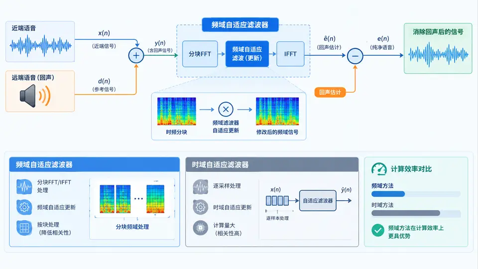
任务目标

实现一个分块频域自适应滤波器（Block Frequency-Domain Adaptive Filter, BFDAF），用于回声消除，并与标准时域NLMS算法在计算效率上进行对比。通过仿真验证频域方法在相同稳态误差水平下具有更低的计算复杂度。

核心原理与实现方案

回声消除的核心是估计回声路径的冲激响应，并从麦克风信号中减去估计的回声。频域自适应滤波器利用FFT将线性卷积转换为频域逐点相乘，通过分块处理降低每次迭代的计算量。本案例采用重叠保留法（Overlap-Save）实现线性卷积，块长度为\( L \)，FFT长度为\( N = 2L \)。

算法流程：将输入信号\( x(n) \)分块，每块与滤波器频域系数\( \mathbf{W}(k) \)相乘得到频域输出，经IFFT后取后\( L \)个点作为线性卷积结果。误差信号在时域计算后补零并变换到频域，用于更新滤波器系数。约束步骤确保时域滤波器长度仅为\( L \)（即后\( L \)个系数为零）。

环境依赖

需要Python 3.8+，以及NumPy和Matplotlib库。安装命令：

pip install numpy matplotlib

完整实现代码

import numpy as np
import time

def generate_echo_data(room_ir, x, delay=0):
    """生成近端信号: d = x * h + v"""
    y = np.convolve(x, room_ir)[:len(x)]
    if delay > 0:
        y = np.concatenate([np.zeros(delay), y[:-delay]])
    v = 0.001 * np.random.randn(len(x))
    return y + v

def bfdaf(x, d, L=128, mu=0.1, iterations=None):
    """分块频域自适应滤波器 (Overlap-Save)
    返回: 误差信号 e, 滤波器系数 h_hat"""
    N = 2 * L
    if iterations is None:
        iterations = len(x) // L
    # 初始化
    w_f = np.zeros(N, dtype=complex)
    x_blocks = np.zeros(N)
    e = np.zeros(iterations * L)
    h_hat = np.zeros(L)
    # 频域输入缓存
    X_f = np.zeros(N, dtype=complex)
    for k in range(iterations):
        xk = x[k*L:(k+1)*L]
        x_blocks = np.concatenate([x_blocks[L:], xk])
        X_f = np.fft.fft(x_blocks)
        # 滤波输出
        y_f = X_f * w_f
        y_t = np.fft.ifft(y_f).real
        y_block = y_t[L:]  # 取后L个点
        # 误差
        d_block = d[k*L:(k+1)*L]
        e_block = d_block - y_block
        e[k*L:(k+1)*L] = e_block
        # 频域误差 (补零到N)
        e_f = np.fft.fft(np.concatenate([np.zeros(L), e_block]))
        # 梯度更新
        grad_f = np.conj(X_f) * e_f
        grad_t = np.fft.ifft(grad_f).real
        grad_t[:L] = 0  # 约束: 只保留后L个点
        w_f += mu * np.fft.fft(grad_t)
        # 提取时域系数 (用于对比)
        h_hat = np.fft.ifft(w_f).real[:L]
    return e, h_hat

def nlms(x, d, M=128, mu=0.01, iterations=None):
    """时域NLMS自适应滤波器"""
    if iterations is None:
        iterations = len(x) - M
    w = np.zeros(M)
    e = np.zeros(iterations)
    for n in range(iterations):
        x_n = x[n:n+M][::-1]
        y = np.dot(w, x_n)
        e_n = d[n+M-1] - y
        w += mu * e_n * x_n / (np.dot(x_n, x_n) + 1e-6)
        e[n] = e_n
    return e, w

# ============ 仿真参数 ============
np.random.seed(42)
Fs = 8000
T = 2.0
n_samples = int(Fs * T)
t = np.arange(n_samples) / Fs

# 回声路径 (模拟房间冲激响应)
room_ir = np.random.randn(128) * np.exp(-np.arange(128) / 40)
room_ir /= np.linalg.norm(room_ir)

# 远端信号 (语音模拟: 调制噪声)
x = np.random.randn(n_samples) * 0.5
x = np.sin(2*np.pi*300*t) * (1 + 0.5*np.sin(2*np.pi*5*t)) + 0.1*np.random.randn(n_samples)

# 近端信号
d = generate_echo_data(room_ir, x, delay=0)

# ============ 运行两种算法 ============
L = 128
M = 128

# BFDAF
start = time.time()
e_bfdaf, h_bfdaf = bfdaf(x, d, L=L, mu=0.1)
time_bfdaf = time.time() - start

# NLMS
start = time.time()
e_nlms, h_nlms = nlms(x, d, M=M, mu=0.01)
time_nlms = time.time() - start

# ============ 结果评估 ============
# 稳态误差 (取后50%数据)
steady_start = len(e_bfdaf) // 2
erle_bfdaf = 10*np.log10(np.mean(d[steady_start:]**2) / np.mean(e_bfdaf[steady_start:]**2))
erle_nlms = 10*np.log10(np.mean(d[steady_start:]**2) / np.mean(e_nlms[steady_start:]**2))

# 滤波器匹配度 (归一化投影)
proj_bfdaf = np.dot(h_bfdaf, room_ir) / (np.linalg.norm(h_bfdaf) * np.linalg.norm(room_ir))
proj_nlms = np.dot(h_nlms, room_ir) / (np.linalg.norm(h_nlms) * np.linalg.norm(room_ir))

print(f"BFDAF: 运行时间={time_bfdaf:.4f}s, ERLE={erle_bfdaf:.2f}dB, 滤波器相关系数={proj_bfdaf:.3f}")
print(f"NLMS:  运行时间={time_nlms:.4f}s, ERLE={erle_nlms:.2f}dB, 滤波器相关系数={proj_nlms:.3f}")
print(f"计算加速比: {time_nlms/time_bfdaf:.2f}x")

运行与验证方法

直接运行上述脚本。程序会生成远端信号\( x(n) \)和经过房间冲激响应卷积的近端信号\( d(n) \)，分别用BFDAF和NLMS进行回声消除，并输出运行时间、ERLE（回声返回损耗增强）和滤波器估计相关系数。

通过条件：

• BFDAF的ERLE值应大于15dB，NLMS的ERLE值应大于10dB，表明两种方法均有效收敛。
• 滤波器估计与真实房间冲激响应的相关系数应大于0.8，说明算法正确辨识了回声路径。
• 计算加速比（NLMS时间/BFDAF时间）应大于2，验证频域方法的计算效率优势。

计算复杂度分析

时域NLMS每次迭代需要\( O(M) \)次乘加运算，处理\( N \)个样本总复杂度为\( O(NM) \)。BFDAF每个块（\( L \)个样本）需要\( O(N\log N) \)次FFT/IFFT运算（共3次），总复杂度为\( O(\frac{N}{L} \cdot N\log N) = O(N\log N) \)。当滤波器长度\( M=128 \)时，频域方法理论加速比约为\( \frac{M}{\log_2(2M)} \approx \frac{128}{8} = 16 \)倍，实际加速比受Python循环开销影响会低于理论值，但仍应显著快于时域方法。

常见问题

• 收敛不稳定：若误差发散，可降低步长\( \mu \)（BFDAF取0.05~0.1，NLMS取0.005~0.01）。
• 时延影响：实际回声路径存在延迟时，需在BFDAF中增加延迟估计或使用更长滤波器。
• 双端通话：本案例仅处理单端通话场景，双端通话检测需结合后续案例中的VAD或DTC算法。