1. Introduction to mesh convergence and tim

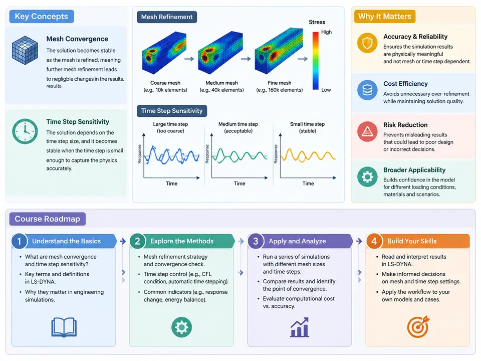
LS-DYNA is an explicit finite element solver, and every result it produces is the product of two independent numerical approximations: the spatial discretization (the mesh) and the temporal discretization (the time step). Neither approximation is "correct" in an absolute sense — both are choices, and both introduce error. Mesh convergence and time step sensitivity are the two disciplines that let an analyst quantify, control, and defend those errors. This chapter establishes the vocabulary, explains why the two topics are inseparable in explicit dynamics, and lays out the roadmap for the rest of the course.

What Mesh Convergence Actually Means

Mesh convergence is the property that a computed quantity of interest (QoI) stops changing meaningfully as the mesh is refined. Formally, if h denotes a characteristic element size and Q(h) the QoI, convergence means that the relative change |Q(h/2) − Q(h)| / |Q(h)| falls below a stated tolerance — commonly 3–5% for engineering work — and stays below it under further refinement. The QoI must be named explicitly: peak von Mises stress, maximum intrusion, reaction force at a specific node, energy absorbed, or first natural frequency. "The mesh is converged" is a meaningless statement without a QoI, a tolerance, and a refinement history.

Two failure modes dominate practice. The first is under-refinement: too few elements across a bending wave, a contact patch, or a stress concentration, so the solution is artificially stiff and the peak stress is under-predicted. The second is non-convergence by singularity: at a sharp re-entrant corner or a point load, the theoretical stress is infinite, so refining the mesh raises the peak stress without bound. In that case the peak nodal stress will never converge, and the analyst must switch to a convergent QoI — a stress averaged over a defined gauge volume, a force, or a displacement — rather than chase an asymptote that does not exist.

What Time Step Sensitivity Means

In LS-DYNA's explicit central-difference scheme, stability is governed by the Courant condition. For a solid element the critical step is approximately

Δt_crit ≈ (L_e / c) ,   c = sqrt(E / ρ)

where L_e is the characteristic element length and c the dilatational wave speed. LS-DYNA computes a per-element estimate and takes the global minimum; the actual step is Δt = TSSFAC × Δt_crit, with TSSFAC defaulting to 0.9 for solid elements. Time step sensitivity is the study of how the results respond to this choice: too large a step and the solution goes unstable (energy grows without bound, elements distort wildly); too small a step and the run becomes needlessly expensive, and in some formulations — notably strain-rate-dependent materials — the step also interacts with the physical time scales being resolved.

The practical consequence is that the time step is not a free knob. It is set by the smallest element in the model, which is usually a deliberate refinement in a contact region or a thin shell. A single 0.5 mm element in a model whose nominal size is 5 mm can cut the step by an order of magnitude and multiply runtime accordingly. This is why mass scaling, selective sub-cycling, and element quality control are core skills rather than afterthoughts.

Why the Two Topics Must Be Studied Together

Refining the mesh changes the time step. Halving h in a solid region halves L_e, halves Δt_crit, and roughly doubles the element count in 2D or multiplies it by eight in 3D — so cost scales between four and sixteen times per refinement level. An analyst who refines the mesh to chase convergence without watching the step will often find the run has become impractical, and may be tempted to compensate with aggressive mass scaling. That compensation changes the inertia of the model and can silently alter the very QoI being converged. The two approximations are coupled through cost and through physics, and the course treats them as a single workflow.

Engineering Relevance

In crashworthiness and impact work, mesh and step choices directly determine whether a design passes or fails a certification load case. An under-refined B-pillar model can under-predict peak intrusion by 10–20%, and an unstable step can produce a "result" that looks plausible in a contour plot but violates energy balance. In drop-test simulation of electronics, the solder-joint stress is governed by elements on the order of 0.1 mm, and the resulting step may be 10–50 ns — a fact that dictates the entire modeling strategy. In metal forming, the through-thickness element count controls springback prediction, while the step controls whether the explicit run is competitive with an implicit solver. Across all of these, the analyst must be able to state, with evidence, why the chosen mesh and step are adequate.

Course Roadmap

The course is organized so that each concept is introduced, then exercised on a reproducible model, then checked against a quantitative criterion. The structure is:

• Foundations (Ch. 1–4): definitions, the Courant condition, element formulations and their effect on Δt_crit, and how LS-DYNA reports the initial and running time step in d3hsp and the message file.
• Mesh convergence methodology (Ch. 5–10): selecting QoIs, refinement ratios, Richardson extrapolation and the Grid Convergence Index, handling singularities, and convergence of contact and energy quantities.
• Time step control (Ch. 11–16): TSSFAC, DT2MS mass scaling, selective mass scaling, *CONTROL_TIMESTEP settings, and diagnosing instability from the energy ratio.
• Coupled workflow (Ch. 17–22): designing a study that varies mesh and step together, cost modeling, and automation with parameterized keyword decks.
• Case studies and verification (Ch. 23–30): crash box, drop test, and forming examples; verification against analytical and experimental data; and documentation of convergence evidence for review.

The diagram below shows how the two approximations feed the same result and where the analyst intervenes.

A First Reproducible Exercise

To make the concepts concrete before the methodology chapters, consider a simple uniaxial bar impact: a 200 mm long, 20 × 20 mm square steel bar (E = 210 GPa, ρ = 7850 kg/m³, ν = 0.3) struck at one end by a 10 m/s velocity pulse, with the far end fixed. The wave speed is c ≈ 5170 m/s, so a 5 mm solid element gives Δt_crit ≈ 0.97 μs and a stable step near 0.87 μs at TSSFAC = 0.9. Build three meshes at 10 mm, 5 mm, and 2.5 mm, run each with the same *CONTROL_TIMESTEP settings, and record the peak axial stress at the fixed end and the time of first arrival. The expected pattern — peak stress rising toward the 1D analytical value and arrival time stabilizing — is the first convergence history the student will produce. If the 2.5 mm run shows growing internal energy or a step collapse in d3hsp, the cause is almost always a single distorted element, and the fix is element quality control, not a smaller TSSFAC.

By the end of this course, the reader should be able to design a convergence study, justify the chosen time step with the Courant condition and an energy check, and present the evidence in a form that survives technical review. The remaining chapters build that capability one component at a time.