1. Energy balance fundamentals in explicit

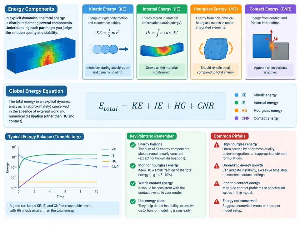
In an explicit dynamics simulation, the solver advances the solution by integrating the equations of motion at very small, stable time increments. Because there is no global stiffness matrix to assemble or invert, the only practical way to judge whether a run is physically trustworthy is to audit the energy bookkeeping. LS-DYNA reports a family of energy quantities at every output interval, and the global energy equation ties them together. Reading that equation correctly is the first diagnostic skill any explicit analyst must acquire: it tells you whether the model is behaving conservatively, whether hourglass modes are contaminating the solution, whether contact is doing spurious work, and whether the time step is small enough to resolve the physics.

The energy quantities LS-DYNA tracks

For a Lagrangian solid or shell model, the principal energy components are:

• Kinetic energy (KE) — the sum over all nodes of ½·m·v². It reflects the momentum in the system and is the quantity that drives deformation when a structure is struck or loaded impulsively.
• Internal energy (IE) — the strain energy stored in the elements plus any energy dissipated by material plasticity, damage, or failure. In LS-DYNA this is accumulated element by element and reported as the sum of elastic and plastic work.
• Hourglass energy (HE) — the energy absorbed by the artificial stiffness or viscosity used to suppress zero-energy hourglass modes in reduced-integration elements. It is a numerical artifact, not a physical quantity, and must be kept small relative to IE.
• Contact energy (CE) — the work done by contact penalty forces, plus energy dissipated by contact friction. It captures the interaction between bodies and is essential when impacts, crushing, or sliding are present.
• External work (EW) — the work done by applied loads, prescribed velocities, body forces, and initial conditions.
• Damping and other dissipation — mass damping, stiffness damping, and any user-defined damping that removes energy from the system.

LS-DYNA also reports a total energy and a sliding interface energy (a component of contact energy), and it tracks the energy of any added mass or initial penetration corrections. The key point is that every joule entering the model must be accounted for somewhere.

The global energy equation

The conservation statement that governs the whole model is:

Equivalently, the energy error or energy ratio reported by LS-DYNA is the difference between the left-hand side and the right-hand side, normalized by the total energy. In a well-behaved explicit run this ratio should stay below roughly 5% and ideally below 1–2%. A steadily growing energy error is a red flag: it usually means the time step is too large, the mesh is badly distorted, contact is unstable, or hourglassing is uncontrolled.

Two conventions matter for consistent interpretation. First, LS-DYNA's sign convention treats external work as positive input and internal dissipation as positive consumption; the equation above is written so that all terms are positive in a conservative system. Second, energies are reported cumulatively from time zero, so a plot of each component versus time is the natural diagnostic view. When you compare runs, always compare the same output interval and the same normalization.

What the balance tells you in practice

The energy equation is not just an accounting identity; each term carries diagnostic meaning. A large and growing hourglass energy relative to internal energy (say above 5–10%) indicates that reduced-integration elements are developing spurious modes — the classic remedy is to switch to fully integrated elements, refine the mesh, or adjust the hourglass control coefficient. A sudden jump in contact energy often signals initial penetration or an unstable penalty stiffness; checking the contact thickness and the penalty scale factor usually resolves it. A kinetic energy that fails to decay when it should, or an internal energy that grows without corresponding external work, points to a time-step or material-model problem.

Worked example: a simple impact bar

Consider a steel bar (length 200 mm, cross-section 20 × 20 mm, density 7850 kg/m³, Young's modulus 210 GPa) striking a rigid wall at 10 m/s. The initial kinetic energy is ½·m·v². With mass m = 0.2 × 0.02 × 0.02 × 7850 ≈ 0.628 kg, KE₀ ≈ 31.4 J. As the bar compresses against the wall, KE converts into IE; at peak compression KE approaches zero and IE approaches 31.4 J, minus any hourglass and contact dissipation. If the run reports HE of 2 J and CE of 0.5 J at that instant, the energy error is (31.4 − 31.4 + 2 + 0.5)/31.4 ≈ 8% — too high, and the hourglass term is the culprit. Reducing the hourglass coefficient or switching to fully integrated elements should bring HE below 1 J and the error under 3%. These numbers are illustrative and should be reproduced in your own model rather than taken as measured results.

Reading the balance over time

Because explicit integration is conditionally stable, the energy balance is also a stability monitor. If the time step exceeds the Courant limit, the solution diverges and the total energy grows without bound — the energy error explodes rather than drifting slowly. In practice, you should inspect the energy plot at the same cadence as the stress and displacement results. A healthy impact simulation shows KE falling smoothly as IE rises, HE staying flat and small, and CE rising only when contact is genuinely active. Any term that steps discontinuously, or any error that climbs monotonically, deserves investigation before the results are used for design decisions.

The global energy equation is therefore both a bookkeeping tool and a physical sanity check. Mastering it early makes every subsequent topic — hourglass control, contact stability, time-step selection — easier to reason about, because each of those topics ultimately shows up as a signature in one of the energy terms.